Algorithmic Trading with MACD in Python
- Nikhil Adithyan

- May 1, 2021
- 15 min read
A step-by-step guide to implementing a powerful strategy

Introduction
In the previous article of this algorithmic trading series, we saw how Bollinger bands can be used to make successful trades. In this article, we are going to discover yet another powerful technical indicator that is considered to be one of the most popular among traders. It’s none other than Moving Average Convergence/Divergence (MACD). We will first understand what this trading indicator is all about then, we will be implementing and backtesting a trading strategy based on this indicator in python to see how well it’s working in the real world. Let’s dive into the article!
MACD
Before moving on to MACD, it is essential to know what Exponential Moving Average (EMA) means. EMA is a type of Moving Average (MA) that automatically allocates greater weighting (nothing but importance) to the most recent data point and lesser weighting to data points in the distant past. For example, a question paper would consist of 10% of one mark questions, 40% of three mark questions, and 50% of long answer questions. From this example, you can observe that we are assigning unique weights to each section of the question paper based on the importance level (probably long answer questions are given more importance than the one mark questions).
Now, MACD is a trend-following leading indicator that is calculated by subtracting two Exponential Moving Averages (one with longer and the other shorter periods). There are three notable components in a MACD indicator.
MACD Line: This line is the difference between two given Exponential Moving Averages. To calculate the MACD line, one EMA with a longer period known as slow length and another EMA with a shorter period known as fast length is calculated. The most popular length of the fast and slow is 12, 26 respectively. The final MACD line values can be arrived at by subtracting the slow length EMA from the fast length EMA. The formula to calculate the MACD line can be represented as follows:
MACD LINE = FAST LENGTH EMA - SLOW LENGTH EMA
Signal Line: This line is the Exponential Moving Average of the MACD line itself for a given period of time. The most popular period to calculate the Signal line is 9. As we are averaging out the MACD line itself, the Signal line will be smoother than the MACD line.
Histogram: As the name suggests, it is a histogram purposely plotted to reveal the difference between the MACD line and the Signal line. It is a great component to be used to identify trends. The formula to calculate the Histogram can be represented as follows:
HISTOGRAM = MACD LINE - SIGNAL LINE
Now that we have an understanding of what MACD exactly is. Let’s gain some intuitions on the trading strategy we are going to build.
About the trading strategy: In this article, we are going to build a simple crossover strategy that will reveal a buy signal whenever the MACD line crosses above the Signal line. Likewise, the strategy will reveal a sell signal whenever the Signal line crosses above the MACD line. Our MACD crossover trading strategy can be represented as follows:
IF MACD LINE > SIGNAL LINE => BUY THE STOCK
IF SIGNAL LINE > MACD LINE => SELL THE STOCK
Before moving on, a note on disclaimer: This article’s sole purpose is to educate people and must be considered as an information piece but not as investment advice or so.
Implementation in Python
After coming across the process of learning what MACD is and gaining some understandings of our trading strategy, we are now set to code our strategy in python and see some interesting results. The coding part is classified into various steps as follows:
1. Importing Packages
2. Extracting Data from Alpha Vantage
3. MACD Calculation
4. MACD Plot
5. Creating the Trading Strategy
6. Plotting the Trading Lists
7. Creating our Position
8. Backtesting
9. SPY ETF Comparison
We will be following the order mentioned in the above list and buckle up your seat belts to follow every upcoming coding part.
Step-1: Importing Packages
Importing the required packages into the python environment is a non-skippable step. The primary packages are going to be Pandas to work with data, NumPy to work with arrays and for complex functions, Matplotlib for plotting purposes, and Requests to make API calls. The secondary packages are going to be Math for mathematical functions and Termcolor for font customization (optional).
Python Implementation:
import requests
import pandas as pd
import numpy as np
from math import floor
from termcolor import colored as cl
import matplotlib.pyplot as plt

plt.rcParams['figure.figsize'] = (20, 10)
plt.style.use('fivethirtyeight')
Now that we have imported all the essential packages into our python environment. Let’s proceed with pulling the historical data of Google with Alpha Vantage’s powerful stock API.
Step-2: Extracting Data from Alpha Vantage
In this step, we are going to pull the historical data of Google using an API endpoint provided by Alpha Vantage. Before that, a note on Alpha Vantage: Alpha Vantage provides free stock APIs through which users can access a wide range of data like real-time updates, and historical data on equities, currencies, and cryptocurrencies. Make sure that you have an account on Alpha Vantage, only then, you will be able to access your secret API key (a crucial element for pulling data using an API).
Python Implementation:
def get_historical_data(symbol, start_date = None):
    api_key = open(r'api_key.txt')
    api_url = f'https://www.alphavantage.co/query?function=TIME_SERIES_DAILY_ADJUSTED&symbol={symbol}&apikey={api_key}&outputsize=full'
    raw_df = requests.get(api_url).json()
    df = pd.DataFrame(raw_df[f'Time Series (Daily)']).T
    df = df.rename(columns = {'1. open': 'open', '2. high': 'high', '3. low': 'low', '4. close': 'close', '5. adjusted close': 'adj close', '6. volume': 'volume'})
    for i in df.columns:
        df[i] = df[i].astype(float)
    df.index = pd.to_datetime(df.index)
    df = df.iloc[::-1].drop(['7. dividend amount', '8. split coefficient'], axis = 1)
    if start_date:
        df = df[df.index >= start_date]
    return df

googl = get_historical_data('GOOGL', '2020-01-01')
googl
Output:

Code Explanation: The first thing we did is to define a function named ‘get_historical_data’ that takes the stock’s symbol (‘symbol’) as a required parameter and the starting date of the historical data (‘start_date’) as an optional parameter. Inside the function, we are defining the API key and the URL and stored them into their respective variable. Next, we are extracting the historical data in JSON format using the ‘get’ function and stored it into the ‘raw_df’ variable. After doing some processes to clean and format the raw JSON data, we are returning it in the form of a clean Pandas dataframe. Finally, we are calling the created function to pull the historic data of Google from the starting of 2020 and stored it into the ‘googl’ variable.
Step-3: MACD Calculation
In this step, we are going to calculate all the components of the MACD indicator from the extracted historical data of Google.
Python Implementation:
def get_macd(price, slow, fast, smooth):
    exp1 = price.ewm(span = fast, adjust = False).mean()
    exp2 = price.ewm(span = slow, adjust = False).mean()
    macd = pd.DataFrame(exp1 - exp2).rename(columns = {'close':'macd'})
    signal = pd.DataFrame(macd.ewm(span = smooth, adjust = False).mean()).rename(columns = {'macd':'signal'})
    hist = pd.DataFrame(macd['macd'] - signal['signal']).rename(columns = {0:'hist'})
    frames =  [macd, signal, hist]
    df = pd.concat(frames, join = 'inner', axis = 1)
    return df

googl_macd = get_macd(googl['close'], 26, 12, 9)
googl_macd.tail()
Output:

Code Explanation: Firstly, we are defining a function named ‘get_macd’ that takes the stock’s price (‘prices’), length of the slow EMA (‘slow’), length of the fast EMA (‘fast’), and the period of the Signal line (‘smooth’).
Inside the function, we are first calculating the fast and slow length EMAs using the ‘ewm’ function provided by Pandas and stored them into the ‘ema1’ and ‘ema2’ variables respectively. Next, we calculated the values of the MACD line by subtracting the slow length EMA from the fast length EMA and stored it into the ‘macd’ variable in the form of a Pandas dataframe. Followed by that, we defined a variable named ‘signal’ to store the values of the Signal line calculated by taking the EMA of the MACD line’s values (‘macd’) for a specified number of periods. Then, we calculated the Histogram values by subtracting the MACD line’s values (‘macd’) from the Signal line’s values (‘signal’) and stored them into the ‘hist’ variable.
Finally, we combined all the calculated values into one dataframe using the ‘concat’ function by the Pandas package and returned the final dataframe. Using the created function, we stored all the MACD components that are calculated from the stock price of Google and stored it into the ‘googl_macd’ variable. From the output, you could see that our dataframe has all the components we discussed before.
Step-4: MACD Plot
In this step, we are going to plot the calculated MACD components to make more sense out of them. Before moving on, it is necessary to know that leading indicators are plotted below the stock prices separately. MACD being a leading indicator needs to be plotted the same way.
Python Implementation:
def plot_macd(prices, macd, signal, hist):
    ax1 = plt.subplot2grid((8,1), (0,0), rowspan = 5, colspan = 1)
    ax2 = plt.subplot2grid((8,1), (5,0), rowspan = 3, colspan = 1)

    ax1.plot(prices)
    ax2.plot(macd, color = 'grey', linewidth = 1.5, label = 'MACD')
    ax2.plot(signal, color = 'skyblue', linewidth = 1.5, label = 'SIGNAL')

    for i in range(len(prices)):
        if str(hist[i])[0] == '-':
            ax2.bar(prices.index[i], hist[i], color = '#ef5350')
        else:
            ax2.bar(prices.index[i], hist[i], color = '#26a69a')

    plt.legend(loc = 'lower right')

plot_macd(googl['close'], googl_macd['macd'], googl_macd['signal'], googl_macd['hist'])
Output:
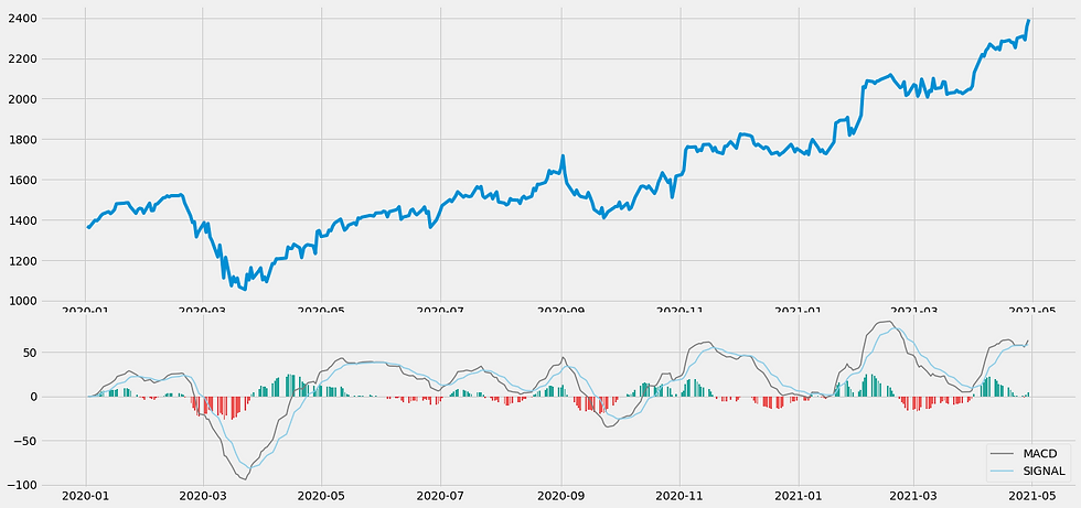
We are not going to dive deep into the code used to produce the above MACD plot instead, we are going to discuss the plot. There are two panels in this plot: the top panel is the plot of Google’s close prices, and the bottom panel is a series of plots of the calculated MACD components. Let’s break and see each and every component.
The first and most visible component in the bottom panel is obviously the plot of the calculated Histogram values. You can notice that the plot turns red whenever the market shows a negative trend and turns green whenever the market reveals a positive trend. This feature of the Histogram plot becomes very handy when it comes to identifying the trend of the market. The Histogram plot spreads larger whenever the difference between the MACD line and the Signal line is huge and it is noticeable that the Histogram plot shrinks at times representing the difference between the two of the other components is comparatively smaller.
The next two components are the MACD line and the Signal line. The MACD line is the grey-colored line plot that shows the difference between the slow length EMA and the fast length EMA of Google’s stock prices. Similarly, the blue-colored line plot is the Signal line that represents the EMA of the MACD line itself. Like we discussed before, the Signal line seems to be more of a smooth-cut version of the MACD line because it is calculated by averaging out the values of the MACD line itself. That’s it about the chart which is shown above as output. Let’s proceed to the next step.
Step-5: Creating the Trading Strategy
In this step, we are going to implement the discussed MACD trading strategy in python.
Python Implementation:
def implement_macd_strategy(prices, data):
    buy_price = []
    sell_price = []
    macd_signal = []
    signal = 0

    for i in range(len(data)):
        if data['macd'][i] > data['signal'][i]:
            if signal != 1:
                buy_price.append(prices[i])
                sell_price.append(np.nan)
                signal = 1
                macd_signal.append(signal)
            else:
                buy_price.append(np.nan)
                sell_price.append(np.nan)
                macd_signal.append(0)
        elif data['macd'][i] < data['signal'][i]:
            if signal != -1:
                buy_price.append(np.nan)
                sell_price.append(prices[i])
                signal = -1
                macd_signal.append(signal)
            else:
                buy_price.append(np.nan)
                sell_price.append(np.nan)
                macd_signal.append(0)
        else:
            buy_price.append(np.nan)
            sell_price.append(np.nan)
            macd_signal.append(0)

    return buy_price, sell_price, macd_signal

buy_price, sell_price, macd_signal = implement_macd_strategy(googl['close'], googl_macd)
Code Explanation: First, we are defining a function named ‘implement_macd_strategy’ which takes the stock prices (‘data’), and MACD data (‘data’) as parameters.
Inside the function, we are creating three empty lists (buy_price, sell_price, and macd_signal) in which the values will be appended while creating the trading strategy.
After that, we are implementing the trading strategy through a for-loop. Inside the for-loop, we are passing certain conditions, and if the conditions are satisfied, the respective values will be appended to the empty lists. If the condition to buy the stock gets satisfied, the buying price will be appended to the ‘buy_price’ list, and the signal value will be appended as 1 representing to buy the stock. Similarly, if the condition to sell the stock gets satisfied, the selling price will be appended to the ‘sell_price’ list, and the signal value will be appended as -1 representing to sell the stock.
Finally, we are returning the lists appended with values. Then, we are calling the created function and stored the values into their respective variables. The list doesn’t make any sense unless we plot the values. So, let’s plot the values of the created trading lists.
Step-6: Plotting the Trading Lists
In this step, we are going to plot the created trading lists to make sense out of them.
Python Implementation:
ax1 = plt.subplot2grid((8,1), (0,0), rowspan = 5, colspan = 1)
ax2 = plt.subplot2grid((8,1), (5,0), rowspan = 3, colspan = 1)

ax1.plot(googl['close'], color = 'skyblue', linewidth = 2, label = 'GOOGL')
ax1.plot(googl.index, buy_price, marker = '^', color = 'green', markersize = 10, label = 'BUY SIGNAL', linewidth = 0)
ax1.plot(googl.index, sell_price, marker = 'v', color = 'r', markersize = 10, label = 'SELL SIGNAL', linewidth = 0)
ax1.legend()
ax1.set_title('GOOGL MACD SIGNALS')
ax2.plot(googl_macd['macd'], color = 'grey', linewidth = 1.5, label = 'MACD')
ax2.plot(googl_macd['signal'], color = 'skyblue', linewidth = 1.5, label = 'SIGNAL')

for i in range(len(googl_macd)):
    if str(googl_macd['hist'][i])[0] == '-':
        ax2.bar(googl_macd.index[i], googl_macd['hist'][i], color = '#ef5350')
    else:
        ax2.bar(googl_macd.index[i], googl_macd['hist'][i], color = '#26a69a')

plt.legend(loc = 'lower right')
plt.show()
Output:

Code Explanation: We are plotting the MACD components along with the buy and sell signals generated by the trading strategy. We can observe that whenever the MACD line crosses above the Signal line, a buy signal is plotted in green color, similarly, whenever the Signal line crosses above the MACD line, a sell signal is plotted in red color. Now, using the trading signals, let’s create our position on the stock.
Step-7: Creating our Position
In this step, we are going to create a list that indicates 1 if we hold the stock or 0 if we don’t own or hold the stock.
Python Implementation:
position = []
for i in range(len(macd_signal)):
    if macd_signal[i] > 1:
        position.append(0)
    else:
        position.append(1)

for i in range(len(googl['close'])):
    if macd_signal[i] == 1:
        position[i] = 1
    elif macd_signal[i] == -1:
        position[i] = 0
    else:
        position[i] = position[i-1]

macd = googl_macd['macd']
signal = googl_macd['signal']
close_price = googl['close']
macd_signal = pd.DataFrame(macd_signal).rename(columns = {0:'macd_signal'}).set_index(googl.index)
position = pd.DataFrame(position).rename(columns = {0:'macd_position'}).set_index(googl.index)

frames = [close_price, macd, signal, macd_signal, position]
strategy = pd.concat(frames, join = 'inner', axis = 1)

strategy
Output:

Code Explanation: First, we are creating an empty list named ‘position’. We are passing two for-loops, one is to generate values for the ‘position’ list to just match the length of the ‘signal’ list. The other for-loop is the one we are using to generate actual position values. Inside the second for-loop, we are iterating over the values of the ‘signal’ list, and the values of the ‘position’ list get appended concerning which condition gets satisfied. The value of the position remains 1 if we hold the stock or remains 0 if we sold or don’t own the stock. Finally, we are doing some data manipulations to combine all the created lists into one dataframe.
From the output being shown, we can see that in the first row our position in the stock has remained 1 (since there isn’t any change in the MACD signal) but our position suddenly turned to 0 as we sold the stock when the MACD trading signal represents a sell signal (-1). Now it’s time to do implement some backtesting process!
Step-8: Backtesting
Before moving on, it is essential to know what backtesting is. Backtesting is the process of seeing how well our trading strategy has performed on the given stock data. In our case, we are going to implement a backtesting process for our MACD trading strategy over the Google stock data.
Python Implementation:
googl_ret = pd.DataFrame(np.diff(googl['close'])).rename(columns = {0:'returns'})
macd_strategy_ret = []

for i in range(len(googl_ret)):
    try:
        returns = googl_ret['returns'][i]*strategy['macd_position'][i]
        macd_strategy_ret.append(returns)
    except:
        pass

macd_strategy_ret_df = pd.DataFrame(macd_strategy_ret).rename(columns = {0:'macd_returns'})

investment_value = 100000
number_of_stocks = floor(investment_value/googl['close'][-1])
macd_investment_ret = []

for i in range(len(macd_strategy_ret_df['macd_returns'])):
    returns = number_of_stocks*macd_strategy_ret_df['macd_returns'][i]
    macd_investment_ret.append(returns)

macd_investment_ret_df = pd.DataFrame(macd_investment_ret).rename(columns = {0:'investment_returns'})
total_investment_ret = round(sum(macd_investment_ret_df['investment_returns']), 2)
profit_percentage = floor((total_investment_ret/investment_value)*100)
print(cl('Profit gained from the MACD strategy by investing $100k in GOOGL : {}'.format(total_investment_ret), attrs = ['bold']))
print(cl('Profit percentage of the MACD strategy : {}%'.format(profit_percentage), attrs = ['bold']))
Output:
Profit gained from the MACD strategy by investing $100k in GOOGL : 38275.02
Profit percentage of the MACD strategy : 38%
Code Explanation: First, we are calculating the returns of the Google stock using the ‘diff’ function provided by the NumPy package and we have stored it as a dataframe into the ‘googl_ret’ variable. Next, we are passing a for-loop to iterate over the values of the ‘googl_ret’ variable to calculate the returns we gained from our MACD trading strategy, and these returns values are appended to the ‘macd_strategy_ret’ list. Next, we are converting the ‘macd_strategy_ret’ list into a dataframe and stored it into the ‘macd_strategy_ret_df’ variable.
Next comes the backtesting process. We are going to backtest our strategy by investing a hundred thousand USD into our trading strategy. So first, we are storing the amount of investment into the ‘investment_value’ variable. After that, we are calculating the number of Google stocks we can buy using the investment amount. You can notice that I’ve used the ‘floor’ function provided by the Math package because, while dividing the investment amount by the closing price of Google stock, it spits out an output with decimal numbers. The number of stocks should be an integer but not a decimal number. Using the ‘floor’ function, we can cut out the decimals. Remember that the ‘floor’ function is way more complex than the ‘round’ function. Then, we are passing a for-loop to find the investment returns followed by some data manipulations tasks.
Finally, we are printing the total return we got by investing a hundred thousand into our trading strategy and it is revealed that we have made an approximate profit of thirty-eight thousand and three hundred USD in one year. That’s not bad! Now, let’s compare our returns with SPY ETF (an ETF designed to track the S&P 500 stock market index) returns.
Step-9: SPY ETF Comparison
This step is optional but it is highly recommended as we can get an idea of how well our trading strategy performs against a benchmark (SPY ETF). In this step, we are going to extract the data of the SPY ETF using the ‘get_historical_data’ function we created and compare the returns we get from the SPY ETF with our MACD strategy returns on Google.
Python Implementation:
def get_benchmark(start_date, investment_value):
    spy = get_historical_data('SPY', start_date)['close']
    benchmark = pd.DataFrame(np.diff(spy)).rename(columns = {0:'benchmark_returns'})

    investment_value = investment_value
    number_of_stocks = floor(investment_value/spy[-1])
    benchmark_investment_ret = []

    for i in range(len(benchmark['benchmark_returns'])):
        returns = number_of_stocks*benchmark['benchmark_returns'][i]
        benchmark_investment_ret.append(returns)

    benchmark_investment_ret_df = pd.DataFrame(benchmark_investment_ret).rename(columns = {0:'investment_returns'})
    return benchmark_investment_ret_df

benchmark = get_benchmark('2020-01-01', 100000)

investment_value = 100000
total_benchmark_investment_ret = round(sum(benchmark['investment_returns']), 2)
benchmark_profit_percentage = floor((total_benchmark_investment_ret/investment_value)*100)
print(cl('Benchmark profit by investing $100k : {}'.format(total_benchmark_investment_ret), attrs = ['bold']))
print(cl('Benchmark Profit percentage : {}%'.format(benchmark_profit_percentage), attrs = ['bold']))
print(cl('MACD Strategy profit is {}% higher than the Benchmark Profit'.format(profit_percentage - benchmark_profit_percentage), attrs = ['bold']))
Output:
Benchmark profit by investing $100k : 22655.22
Benchmark Profit percentage : 22%
MACD Strategy profit is 16% higher than the Benchmark Profit
Code Explanation: The code used in this step is almost similar to the one used in the previous backtesting step but, instead of investing in Google, we are investing in SPY ETF by not implementing any trading strategies. From the output, we can see that our MACD trading strategy has outperformed the SPY ETF by 16%. That’s great!
Final Thoughts!
MACD is one of the most powerful strategies present out there and it can be highly efficient when applied to the real-world market. If you decide to use MACD in the real-world market, there is one important thing to keep in mind. MACD has the tendency to reveal false trading signals. So, it is highly recommended to use a technical indicator in addition to MACD to cross verify whether the represented signal actually is an authentic trading signal. We have not covered using multiple indicators to build a MACD strategy as the sole purpose of the article is to just understand what MACD is and how it can be implemented using python.
You can also notice that the stock we used to implement our MACD trading strategy is randomly chosen which is not a great approach. Ways to deal with picking stocks can be done by a quantitative approach or an ML algorithm-based approach. This can significantly improve our results. That’s it! Hope you learned something useful from this article. And, if you forgot to follow some of the coding parts, don’t worry! I’ve provided the full source at the end of the article.
Full code:
import requests
import pandas as pd
import numpy as np
from math import floor
from termcolor import colored as cl
import matplotlib.pyplot as plt

plt.rcParams['figure.figsize'] = (20, 10)
plt.style.use('fivethirtyeight')

def get_historical_data(symbol, start_date = None):
    api_key = open(r'api_key.txt')
    api_url = f'https://www.alphavantage.co/query?function=TIME_SERIES_DAILY_ADJUSTED&symbol={symbol}&apikey={api_key}&outputsize=full'
    raw_df = requests.get(api_url).json()
    df = pd.DataFrame(raw_df[f'Time Series (Daily)']).T
    df = df.rename(columns = {'1. open': 'open', '2. high': 'high', '3. low': 'low', '4. close': 'close', '5. adjusted close': 'adj close', '6. volume': 'volume'})
    for i in df.columns:
        df[i] = df[i].astype(float)
    df.index = pd.to_datetime(df.index)
    df = df.iloc[::-1].drop(['7. dividend amount', '8. split coefficient'], axis = 1)
    if start_date:
        df = df[df.index >= start_date]
    return df

googl = get_historical_data('GOOGL', '2020-01-01')
googl

def get_macd(price, slow, fast, smooth):
    exp1 = price.ewm(span = fast, adjust = False).mean()
    exp2 = price.ewm(span = slow, adjust = False).mean()
    macd = pd.DataFrame(exp1 - exp2).rename(columns = {'close':'macd'})
    signal = pd.DataFrame(macd.ewm(span = smooth, adjust = False).mean()).rename(columns = {'macd':'signal'})
    hist = pd.DataFrame(macd['macd'] - signal['signal']).rename(columns = {0:'hist'})
    frames =  [macd, signal, hist]
    df = pd.concat(frames, join = 'inner', axis = 1)
    return df

googl_macd = get_macd(googl['close'], 26, 12, 9)
googl_macd

def plot_macd(prices, macd, signal, hist):
    ax1 = plt.subplot2grid((8,1), (0,0), rowspan = 5, colspan = 1)
    ax2 = plt.subplot2grid((8,1), (5,0), rowspan = 3, colspan = 1)

    ax1.plot(prices)
    ax2.plot(macd, color = 'grey', linewidth = 1.5, label = 'MACD')
    ax2.plot(signal, color = 'skyblue', linewidth = 1.5, label = 'SIGNAL')

    for i in range(len(prices)):
        if str(hist[i])[0] == '-':
            ax2.bar(prices.index[i], hist[i], color = '#ef5350')
        else:
            ax2.bar(prices.index[i], hist[i], color = '#26a69a')

    plt.legend(loc = 'lower right')

plot_macd(googl['close'], googl_macd['macd'], googl_macd['signal'], googl_macd['hist'])

def implement_macd_strategy(prices, data):
    buy_price = []
    sell_price = []
    macd_signal = []
    signal = 0

    for i in range(len(data)):
        if data['macd'][i] > data['signal'][i]:
            if signal != 1:
                buy_price.append(prices[i])
                sell_price.append(np.nan)
                signal = 1
                macd_signal.append(signal)
            else:
                buy_price.append(np.nan)
                sell_price.append(np.nan)
                macd_signal.append(0)
        elif data['macd'][i] < data['signal'][i]:
            if signal != -1:
                buy_price.append(np.nan)
                sell_price.append(prices[i])
                signal = -1
                macd_signal.append(signal)
            else:
                buy_price.append(np.nan)
                sell_price.append(np.nan)
                macd_signal.append(0)
        else:
            buy_price.append(np.nan)
            sell_price.append(np.nan)
            macd_signal.append(0)

    return buy_price, sell_price, macd_signal

buy_price, sell_price, macd_signal = implement_macd_strategy(googl['close'], googl_macd)

ax1 = plt.subplot2grid((8,1), (0,0), rowspan = 5, colspan = 1)
ax2 = plt.subplot2grid((8,1), (5,0), rowspan = 3, colspan = 1)

ax1.plot(googl['close'], color = 'skyblue', linewidth = 2, label = 'GOOGL')
ax1.plot(googl.index, buy_price, marker = '^', color = 'green', markersize = 10, label = 'BUY SIGNAL', linewidth = 0)
ax1.plot(googl.index, sell_price, marker = 'v', color = 'r', markersize = 10, label = 'SELL SIGNAL', linewidth = 0)
ax1.legend()
ax1.set_title('GOOGL MACD SIGNALS')
ax2.plot(googl_macd['macd'], color = 'grey', linewidth = 1.5, label = 'MACD')
ax2.plot(googl_macd['signal'], color = 'skyblue', linewidth = 1.5, label = 'SIGNAL')

for i in range(len(googl_macd)):
    if str(googl_macd['hist'][i])[0] == '-':
        ax2.bar(googl_macd.index[i], googl_macd['hist'][i], color = '#ef5350')
    else:
        ax2.bar(googl_macd.index[i], googl_macd['hist'][i], color = '#26a69a')

plt.legend(loc = 'lower right')
plt.show()

position = []
for i in range(len(macd_signal)):
    if macd_signal[i] > 1:
        position.append(0)
    else:
        position.append(1)

for i in range(len(googl['close'])):
    if macd_signal[i] == 1:
        position[i] = 1
    elif macd_signal[i] == -1:
        position[i] = 0
    else:
        position[i] = position[i-1]

macd = googl_macd['macd']
signal = googl_macd['signal']
close_price = googl['close']
macd_signal = pd.DataFrame(macd_signal).rename(columns = {0:'macd_signal'}).set_index(googl.index)
position = pd.DataFrame(position).rename(columns = {0:'macd_position'}).set_index(googl.index)

frames = [close_price, macd, signal, macd_signal, position]
strategy = pd.concat(frames, join = 'inner', axis = 1)

strategy

googl_ret = pd.DataFrame(np.diff(googl['close'])).rename(columns = {0:'returns'})
macd_strategy_ret = []

for i in range(len(googl_ret)):
    try:
        returns = googl_ret['returns'][i]*strategy['macd_position'][i]
        macd_strategy_ret.append(returns)
    except:
        pass

macd_strategy_ret_df = pd.DataFrame(macd_strategy_ret).rename(columns = {0:'macd_returns'})

investment_value = 100000
number_of_stocks = floor(investment_value/googl['close'][-1])
macd_investment_ret = []

for i in range(len(macd_strategy_ret_df['macd_returns'])):
    returns = number_of_stocks*macd_strategy_ret_df['macd_returns'][i]
    macd_investment_ret.append(returns)

macd_investment_ret_df = pd.DataFrame(macd_investment_ret).rename(columns = {0:'investment_returns'})
total_investment_ret = round(sum(macd_investment_ret_df['investment_returns']), 2)
profit_percentage = floor((total_investment_ret/investment_value)*100)
print(cl('Profit gained from the MACD strategy by investing $100k in GOOGL : {}'.format(total_investment_ret), attrs = ['bold']))
print(cl('Profit percentage of the MACD strategy : {}%'.format(profit_percentage), attrs = ['bold']))

def get_benchmark(start_date, investment_value):
    spy = get_historical_data('SPY', start_date)['close']
    benchmark = pd.DataFrame(np.diff(spy)).rename(columns = {0:'benchmark_returns'})

    investment_value = investment_value
    number_of_stocks = floor(investment_value/spy[-1])
    benchmark_investment_ret = []

    for i in range(len(benchmark['benchmark_returns'])):
        returns = number_of_stocks*benchmark['benchmark_returns'][i]
        benchmark_investment_ret.append(returns)

    benchmark_investment_ret_df = pd.DataFrame(benchmark_investment_ret).rename(columns = {0:'investment_returns'})
    return benchmark_investment_ret_df

benchmark = get_benchmark('2020-01-01', 100000)

investment_value = 100000
total_benchmark_investment_ret = round(sum(benchmark['investment_returns']), 2)
benchmark_profit_percentage = floor((total_benchmark_investment_ret/investment_value)*100)
print(cl('Benchmark profit by investing $100k : {}'.format(total_benchmark_investment_ret), attrs = ['bold']))
print(cl('Benchmark Profit percentage : {}%'.format(benchmark_profit_percentage), attrs = ['bold']))
print(cl('MACD Strategy profit is {}% higher than the Benchmark Profit'.format(profit_percentage - benchmark_profit_percentage), attrs = ['bold']))


Amazing work Nikhil! All the best!
Good One Nikhil
With so much technical points involved, you have neatly presented, the subject, so that people like me,with no technical knowledge,can easily understand. Good work
It's very nice that you're clearly reinforcing the objective of the article in the"final thoughts" section.