How to Use MCP to Build A Personal Financial Assistant
- Nikhil Adithyan

- Mar 6
- 20 min read
A Python guide to using MCPs

LLMs are great at writing market commentary. The problem is they can sound confident even when they have not looked at any data. That’s fine for casual chat. It’s not fine if you’re building a feature for a product, an internal tool, or anything a user might rely on.
In this guide, we’ll build a small financial assistant that answers by fetching real data through MCP (Model Context Protocol), then computing the numbers in Python. The LLM’s job is only to narrate the computed facts. It does not invent metrics, and it does not do the math.
By the end, you’ll have two outputs you can actually plug into a product flow. A single-ticker market brief, and a watchlist snapshot that compares multiple tickers on volatility and drawdown, with the tool calls traced so you can see exactly what data was used.
What is MCP: How it changes the integration story

MCP (Model Context Protocol) is basically a standard way for an LLM app to discover and call external tools. Instead of hardcoding a bunch of function schemas or building custom connectors per framework, you plug into an MCP server and the tools become “available” in a consistent format.
For product teams, this matters because it reduces integration churn. Tool discovery is predictable, you’re not rewriting wrappers every time your stack changes, and you get a clean separation between the model and the data layer. In our case, that data layer is EODHD’s MCP server, which exposes market data tools the assistant can call whenever it needs prices or fundamentals.
One important clarification for this tutorial. We’re using MCP purely as the data access layer. The model does not decide which tools to call or what parameters to pass. We do that deterministically in Python, then hand the model a facts object and let it write the narrative. This keeps the output grounded and makes the system much easier to trust and debug.
Architecture: The “narrator” pattern
Here’s the architecture we’re using in this guide.
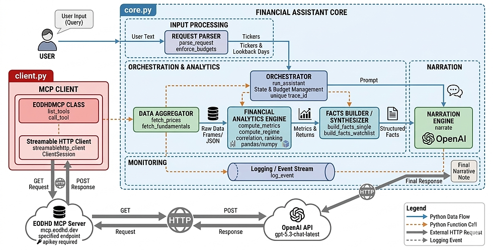
The idea is simple. We separate “getting facts” from “writing words”. The model only does the second part.
First, the user asks a question like “Give me a 30-day brief for AAPL” or “Compare TSLA, NVDA, AMZN over the last 60 days”. That raw text goes into a tiny parser. The parser is intentionally boring. It only extracts what the system needs to operate. A list of tickers and a lookback window.
Once we have tickers and dates, we fetch data through MCP. In this case, MCP is connected to EODHD’s MCP server. So instead of the assistant guessing prices or fundamentals, it calls tools like “get historical prices” and “get fundamentals”. At this point we have raw data. Nothing has been computed yet, and the model has not written a single sentence.
Then Python takes over. This is where we compute everything deterministic. Returns, volatility, max drawdown, trend slope, and a simple volatility regime label. For watchlists, we align returns and compute correlation. These numbers are the backbone of the output. If you rerun the same query with the same window, you should get the same metrics.
Only after that do we involve the LLM. We pass it a compact facts object. It contains the metrics we computed, plus a few clean fundamentals fields. The prompt is strict. Use only these facts. No extra numbers. No guessing. The model’s job is to turn the facts into a clean note that feels like something a product would show.
Finally, the assistant returns a structured response object. Not just text. You get:
answer (the narrative)
metrics (the exact computed numbers)
data_used (tickers, date range, and which tools were called)
tool_trace_id (a trace id you can log, debug, or attach to monitoring)
This pattern is B2B-friendly for a very practical reason. It reduces hallucinations because the model isn’t doing analysis. It makes numbers repeatable because Python computes them. And it’s easy to audit because you can always show what data was fetched, what window was used, and which tool calls happened.
Step 1. MCP client wrapper (client.py)
Before we touch any “assistant logic”, we need one thing. A tiny MCP client wrapper that can connect to EODHD’s MCP server and call tools reliably. That’s it.
This file does three jobs:
opens a streamable HTTP MCP session
calls a tool with a timeout and a small retry loop
returns the tool output plus a small metadata object we can later attach to logs and traces
Here’s the complete client.py.
import time
import asyncio

from mcp import ClientSession
from mcp.client.streamable_http import streamablehttp_client

class EODHDMCP:
    def __init__(self, apikey, base_url=None):
        self.apikey = apikey
        self.base_url = base_url or "https://mcp.eodhd.dev/mcp"
        self._tools = None

    def _url(self):
        return f"{self.base_url}?apikey={self.apikey}"

    def _open(self):
        return streamablehttp_client(self._url())

    async def list_tools(self):
        if self._tools is not None:
            return self._tools

        async with self._open() as (read, write, _):
            async with ClientSession(read, write) as s:
                await s.initialize()
                resp = await s.list_tools()
                self._tools = [t.name for t in resp.tools]
                return self._tools

    async def call_tool(self, name, args, trace_id, timeout_s=25, retries=1):
        last = None

        for attempt in range(retries + 1):
            t0 = time.time()
            try:
                async with self._open() as (read, write, _):
                    async with ClientSession(read, write) as s:
                        await s.initialize()
                        out = await asyncio.wait_for(s.call_tool(name, args), timeout=timeout_s)
                        dt = time.time() - t0
                        meta = {"trace_id": trace_id, "tool": name, "args": args, "latency_s": round(dt, 3)}
                        return out, meta
            except Exception as e:
                last = e
                if attempt < retries:
                    await asyncio.sleep(0.25)

        raise last
How this works:
streamablehttp_client(self._url()) opens a streamable HTTP connection to the MCP server URL. The URL includes your API key as a query param, so the server can authenticate.
list_tools() is just a convenience. It asks the server which tools exist and caches the names in memory so you don’t fetch them repeatedly.
call_tool() is the workhorse. It opens a session, initializes it, calls a tool with call_tool(name, args), and wraps the result with a meta object.
That meta object is important later. It lets you trace which tool was called, with which params, how long it took, and which request it belonged to (trace_id).
Next, we’ll build the core runner in core.py. This is where we parse the user’s request, fetch prices and fundamentals via MCP, compute metrics in Python, and then hand the facts to the LLM for narration.
Step 2. The assistant core (core.py)
This is where the assistant actually becomes “real”. client.py was just a connector. Here we decide what data to fetch, how much to fetch, how to compute the numbers, and what we hand to the model for narration.
i. Budgets and trace logging
When you build anything that calls real tools, you want limits. Not because you don’t trust your code. Because without limits, one messy prompt can easily turn into an expensive, slow request.
In our case, we cap:
how far back we’ll fetch data (MAX_LOOKBACK_DAYS)
how many tool calls we allow per request (MAX_TOOL_CALLS)
how many tickers we’ll accept in one query (MAX_TICKERS)
And we log a few events so we can always debug what happened later.
Here’s the top part of core.py for that.
import json
import re
import time
import uuid
from datetime import date, timedelta
from openai import OpenAI
import numpy as np
import pandas as pd
import asyncio
from client import EODHDMCP

EODHD_API_KEY = "YOUR EODHD API KEY"
MCP_BASE_URL = "https://mcp.eodhd.dev/mcp"

MAX_LOOKBACK_DAYS = 365
MAX_TOOL_CALLS = 6
MAX_TICKERS = 5

mcp = EODHDMCP(EODHD_API_KEY, base_url=MCP_BASE_URL)
oa = OpenAI(api_key = "OPENAI API KEY")
NARRATION_MODEL = "gpt-5.3-chat-latest"

def log_event(event, trace_id, **k):
    payload = {"event": event, "trace_id": trace_id, "ts": round(time.time(), 3)}
    payload.update(k)
    print(json.dumps(payload, default=str))
What’s going on here:
MAX_LOOKBACK_DAYS, MAX_TOOL_CALLS, MAX_TICKERS are basically your safety rails. We’ll enforce them later, right after parsing the user query.
trace_id is a small id we generate per request. Every log line includes it, so when something breaks, you can reconstruct the exact flow for that request.
log_event() prints one JSON line. Nothing fancy. But it’s enough for debugging and it also looks very similar to how real systems emit traces.
Note: Make sure to replace YOUR EODHD API KEY with your actual EODHD API key. If you don’t have one, you can obtain it by creating an EODHD developer account.
ii. Parsing the request
This part is intentionally not “smart”. We’re not doing NLP. We’re not letting the model interpret the query. We just want to extract two things in a predictable way:
tickers
lookback window
That’s it.
The benefit of keeping it dumb is that the behavior is stable. If the query is messy, we still do something consistent, and the rest of the pipeline remains controllable.
Here are the two functions.
def parse_request(text):
    t = (text or "").upper()

    raw = re.findall(r"\b[A-Z]{1,5}\b", t)

    bad = {
        "I","A","AN","THE","AND","OR","TO","FOR","OF","IN","ON","BY","WITH","ME","WE","US",
        "GIVE","DAY","DAYS","BRIEF","COMPARE","RANK","OVER","LAST","TREND","VOL","VOLATILITY",
        "DRAWDOWN","FLAG","RISKS","RISK","PLUS","MAX","MIN","LOOKBACK"
    }

    tickers = []
    for x in raw:
        if x in bad:
            continue
        if len(x) < 2:
            continue
        if x not in tickers:
            tickers.append(x)

    days = 30

    if "LAST" in t:
        after = t.split("LAST", 1)[1]
        m = re.search(r"\d{1,4}", after)
        if m:
            days = int(m.group(0))

    return tickers, days

def enforce_budgets(tickers, lookback_days):
    if lookback_days < 1:
        lookback_days = 1
    if lookback_days > MAX_LOOKBACK_DAYS:
        lookback_days = MAX_LOOKBACK_DAYS

    tickers = tickers[:MAX_TICKERS]

    return tickers, lookback_days
How to read this:
re.findall(r"\b[A-Z]{1,5}\b", t) pulls out every short uppercase token. That’s our crude “ticker candidate” list.
The bad set is just a blacklist of common words that show up in prompts but are obviously not tickers.
We keep unique tickers in order, because the first ticker becomes the “base” for correlation in the watchlist demo.
Lookback is simple. Default is 30 days. If the query contains “last …”, we grab the first number after “LAST”. That avoids regex edge cases with punctuation.
Then enforce_budgets() clamps everything so one request can’t ask for 500 tickers or a 10-year window.
Next, we’ll wire these parsed values into a request state and start making actual MCP calls for prices and fundamentals.
iii. Tool wrappers: Prices and fundamentals
Now we’re at the point where the assistant actually touches data.
These two functions do the same job in different ways:
fetch_prices() calls the MCP tool for historical prices, then normalizes the output into a tiny DataFrame with just date and close.
fetch_fundamentals() calls the MCP tool for fundamentals and returns the JSON.
We also keep a small state object per request. It tracks tool calls and keeps a trace of what was called. That’s how we later produce the data_used block in the final response.
Here’s the code:
def new_state():
    return {"tool_calls": 0, "tool_trace": [], "rows": {}}

def _bump(state, meta):
    state["tool_calls"] += 1
    state["tool_trace"].append(meta)
    if state["tool_calls"] > MAX_TOOL_CALLS:
        raise RuntimeError("tool call budget exceeded")

def _as_json_text(out):
    if isinstance(out, str):
        return out
    if hasattr(out, "content"):
        try:
            return out.content[0].text
        except Exception:
            pass
    return str(out)

async def fetch_prices(ticker, start_date, end_date, trace_id, state):
    args = {
        "ticker": ticker,
        "start_date": start_date,
        "end_date": end_date,
        "period": "d",
        "order": "a",
        "fmt": "json",
    }

    out, meta = await mcp.call_tool("get_historical_stock_prices", args, trace_id)
    txt = _as_json_text(out)

    _bump(state, meta)

    data = json.loads(txt)
    if isinstance(data, dict) and data.get("error"):
        raise RuntimeError(data["error"])

    df = pd.DataFrame(data)
    if df.empty:
        return df

    cols = [c for c in ["date", "close"] if c in df.columns]
    df = df[cols].copy()
    df["ticker"] = ticker

    state["rows"][f"{meta['tool']}:{ticker}"] = len(df)
    return df

async def fetch_fundamentals(ticker, trace_id, state):
    args = {
        "ticker": ticker,
        "include_financials": False,
        "fmt": "json",
    }

    out, meta = await mcp.call_tool("get_fundamentals_data", args, trace_id)
    txt = _as_json_text(out)

    _bump(state, meta)

    data = json.loads(txt)
    if isinstance(data, dict) and data.get("error"):
        raise RuntimeError(data["error"])

    return data
What’s happening here:
_bump() is the budget guard. Every time we make a tool call, we increment the counter and store the tool metadata. If we cross the budget, we fail fast.
meta comes from client.py. It contains tool, args, and latency. That’s enough to trace “what did we call and how long did it take”.
_as_json_text() is there because MCP tool results are not always plain strings. Sometimes it’s an object with .content. This helper just tries to extract the text cleanly.
In fetch_prices(), we intentionally keep only date and close. That’s not because OHLC is useless. It’s because this tutorial’s metrics only need closes. Fewer columns means simpler code, smaller payloads, and fewer chances to break.
Next, we’ll compute the actual metrics. This is where the assistant stops being “an API caller” and starts producing something useful.
iv. Deterministic metrics
This is the most important design choice in the whole build. The model never computes numbers. Python does.
So for every ticker, we compute a small set of metrics that are easy to explain and are actually useful in a “market brief” style output:
total return over the window
realized volatility (daily and annualized)
max drawdown (worst peak-to-trough fall)
a simple trend slope (so we can say “mild uptrend” or “downtrend” without vibes)
a lightweight regime label (low, mid, high volatility)
Here’s the code.
def compute_metrics(prices_df):
    if prices_df is None or prices_df.empty:
        return {}

    df = prices_df.copy()
    df["date"] = pd.to_datetime(df["date"], errors="coerce")
    df = df.dropna(subset=["date"]).sort_values("date")

    close = pd.to_numeric(df["close"], errors="coerce").dropna()
    if close.empty:
        return {}

    rets = close.pct_change().dropna()

    out = {}

    # realized vol (daily), annualize with sqrt(252)
    if not rets.empty:
        out["vol_daily"] = float(rets.std())
        out["vol_annualized"] = float(rets.std() * np.sqrt(252))
        out["ret_total"] = float((close.iloc[-1] / close.iloc[0]) - 1.0)

    # max drawdown
    peak = close.cummax()
    dd = (close / peak) - 1.0
    out["max_drawdown"] = float(dd.min())

    # simple trend score
    logp = np.log(close.values)
    x = np.arange(len(logp))
    if len(logp) >= 3:
        slope = np.polyfit(x, logp, 1)[0]
        out["trend_slope"] = float(slope)
    else:
        out["trend_slope"] = 0.0

    # basic helpers
    out["n_points"] = int(len(close))
    out["start_close"] = float(close.iloc[0])
    out["end_close"] = float(close.iloc[-1])

    return out

def compute_regime(prices_df, window=20):
    # cheap regime label, based on rolling vol percentile
    if prices_df is None or prices_df.empty:
        return {"regime": "unknown"}

    df = prices_df.copy()
    df["date"] = pd.to_datetime(df["date"], errors="coerce")
    df = df.dropna(subset=["date"]).sort_values("date")

    close = pd.to_numeric(df["close"], errors="coerce").dropna()
    if close.empty:
        return {"regime": "unknown"}

    rets = close.pct_change()
    rv = rets.rolling(window).std()

    last = rv.dropna()
    if last.empty:
        return {"regime": "unknown"}

    cur = float(last.iloc[-1])
    p80 = float(last.quantile(0.8))
    p50 = float(last.quantile(0.5))

    if cur >= p80:
        reg = "high_vol"
    elif cur >= p50:
        reg = "mid_vol"
    else:
        reg = "low_vol"

    return {"regime": reg, "rolling_vol": cur, "window": int(window)}
How to think about these calculations:
Total return is just end / start - 1. It’s the simplest “did it go up or down” number.
Volatility here is realized volatility of daily returns. That’s just the standard deviation of daily % changes. We annualize it using sqrt(252) because markets have roughly 252 trading days.
Max drawdown tells you how bad the worst dip was during the window. It’s often more meaningful than return when you’re writing a quick risk note.
Trend slope is intentionally simple. We fit a straight line to log prices. If the slope is positive, it’s generally drifting up. If it’s negative, it’s drifting down.
Regime label is not a fancy model. It just says “compared to its own recent rolling volatility, are we currently in a high, medium, or low vol phase”.
The main point is this. These numbers are deterministic. If the assistant says “max drawdown was -13%”, you can trace it back to the exact close series that produced it.
Next, we’ll handle the watchlist side. That means aligning returns across tickers, computing correlation, and generating a ranked snapshot.
v. Watchlist utilities
Once you have more than one ticker, you want two extra things:
a quick ranking so you can say “this is the riskiest name in the basket”
a correlation snapshot so you can see what’s moving together
The only “gotcha” with correlation is dates. If TSLA has 41 price points and NVDA has 39 because of missing days, you can’t just correlate blindly. You need the returns lined up on the same dates first. That’s what align_returns() does.
Here’s the code:
def align_returns(price_frames):
    if not price_frames:
        return pd.DataFrame()

    parts = []
    for df in price_frames:
        if df is None or df.empty:
            continue
        x = df.copy()
        x["date"] = pd.to_datetime(x["date"], errors="coerce")
        x = x.dropna(subset=["date"])
        x["close"] = pd.to_numeric(x["close"], errors="coerce")
        x = x.dropna(subset=["close"])
        x = x.sort_values("date")
        x["ret"] = x["close"].pct_change()
        x = x.dropna(subset=["ret"])
        parts.append(x[["date", "ticker", "ret"]])

    if not parts:
        return pd.DataFrame()

    allr = pd.concat(parts, ignore_index=True)
    wide = allr.pivot(index="date", columns="ticker", values="ret").dropna(how="any")
    return wide


def corr_summary(ret_wide, base_ticker, top_n=3):
    if ret_wide is None or ret_wide.empty:
        return []

    if base_ticker not in ret_wide.columns:
        return []

    c = ret_wide.corr()[base_ticker].dropna()
    c = c.drop(labels=[base_ticker], errors="ignore")
    if c.empty:
        return []

    out = []
    for k, v in c.sort_values(ascending=False).head(top_n).items():
        out.append({"ticker": k, "corr": float(v)})

    return out


def rank_watchlist(metrics_by_ticker):
    rows = []
    for t, m in metrics_by_ticker.items():
        if not m:
            continue
        rows.append({
            "ticker": t,
            "vol_annualized": m.get("vol_annualized"),
            "max_drawdown": m.get("max_drawdown"),
            "ret_total": m.get("ret_total"),
            "trend_slope": m.get("trend_slope"),
        })

    if not rows:
        return pd.DataFrame()

    df = pd.DataFrame(rows)
    df = df.sort_values(["vol_annualized", "max_drawdown"], ascending=[False, True])
    return df.reset_index(drop=True)
What’s happening here:
align_returns() takes a list of price DataFrames, computes daily returns for each, then pivots them into a wide table like: date -> TSLA.US, NVDA.US, AMZN.US
We drop rows where any ticker is missing, because correlation only makes sense when the returns are aligned on the same dates.
corr_summary() is a compact “who moves with whom” helper. We pick one base ticker, compute correlations against everything else, then grab the top few. For a watchlist widget, that’s usually enough.
rank_watchlist() is the ranking logic for the snapshot. We sort primarily by annualized volatility, and use drawdown as a secondary risk indicator. You could choose different ranking logic. The point is to keep it deterministic and explainable.
Next, we’ll build the facts objects and narration layer. That’s where we enforce the “model is just a narrator” contract.
vi. Facts object and narration
This is where the “narrator pattern” becomes real.
Up to this point, we’ve done everything with MCP and Python. We fetched prices and fundamentals from EODHD, we computed metrics, we aligned returns. Now we need one clean object that represents “the truth” for this request.
That’s what the facts object is.
The rule is simple.
facts contains only things we actually fetched or computed.
The model never sees raw market data. It sees the cleaned facts.
The model is told to write using only those facts, and not to invent any numbers.
Here are the functions that build those facts objects for the two demos, plus the narration function.
def build_facts_single(ticker, lookback_days, metrics, regime, fundamentals):
    # keep this compact. LLM will narrate from this later
    out = {
        "type": "single_ticker_brief",
        "ticker": ticker,
        "lookback_days": int(lookback_days),
        "metrics": metrics,
        "regime": regime,
    }

    if isinstance(fundamentals, dict):
        gen = fundamentals.get("General", {}) or {}
        highlights = {
            "name": gen.get("Name"),
            "exchange": gen.get("Exchange"),
            "sector": gen.get("Sector"),
            "industry": gen.get("Industry"),
            "market_cap": gen.get("MarketCapitalization"),
            "pe": gen.get("PERatio"),
            "beta": gen.get("Beta"),
            "div_yield": gen.get("DividendYield"),
            }
        out["fundamentals"] = {k: v for k, v in highlights.items() if v is not None}

    return out


def build_facts_watchlist(tickers, lookback_days, rank_df, corr_bits, metrics_by_ticker):
    out = {
        "type": "watchlist_snapshot",
        "tickers": tickers,
        "lookback_days": int(lookback_days),
        "ranking": rank_df.to_dict(orient="records") if isinstance(rank_df, pd.DataFrame) else [],
        "correlation": corr_bits,
        "metrics_by_ticker": metrics_by_ticker,
    }
    return out


def narrate(facts):
    prompt = (
        "Write a short, product-ready market note using ONLY the facts below.\n"
        "No guessing. No extra numbers. If something is missing, say it's missing.\n"
        "Keep it tight and readable.\n\n"
        f"FACTS:\n{json.dumps(facts, indent=2, default=str)}"
    )

    r = oa.responses.create(
        model=NARRATION_MODEL,
        input=[{"role": "user", "content": prompt}],
    )

    try:
        return r.output_text
    except Exception:
        return str(r)
What’s happening here:
build_facts_single() takes the ticker, window, computed metrics, the vol regime label, and the fundamentals payload. But it doesn’t dump the entire fundamentals JSON. It picks a handful of fields from the General section and only keeps what exists. That keeps the prompt tight and the output predictable.
build_facts_watchlist() is the same idea but for multiple tickers. It passes the ranking table, correlation notes, and per-ticker metrics.
narrate() is basically “convert this facts object into human-friendly text”. The prompt is strict on purpose. If the model can only see these facts, it cannot hallucinate numbers outside them.
One small implementation detail. narrate() is a normal blocking function, while everything else is async. That’s why later, inside run_assistant(), we call it with await asyncio.to_thread(...) so it doesn’t block the async flow.
vii. The orchestration function (run_assistant())
This is the piece that ties everything together. It does four things in order:
create a trace id and log the request
parse tickers and lookback, then clamp them to budgets
fetch EODHD data via MCP and compute metrics in Python
call the model to narrate the facts, then return a structured response
Here’s the function:
def _dates_from_lookback(lookback_days):
    end = date.today()
    start = end - timedelta(days=int(lookback_days))
    return start.isoformat(), end.isoformat()

async def run_assistant(user_text, mode="auto"):
    trace_id = uuid.uuid4().hex[:10]
    log_event("request_started", trace_id, text=user_text, mode=mode)

    tickers, lookback = parse_request(user_text)
    tickers, lookback = enforce_budgets(tickers, lookback)

    if not tickers:
        return {
            "answer": "no tickers found in request",
            "metrics": {},
            "data_used": {},
            "tool_trace_id": trace_id,
        }

    log_event("parsed", trace_id, tickers=tickers, lookback_days=lookback)

    start_date, end_date = _dates_from_lookback(lookback)
    state = new_state()

    if mode == "auto":
        mode = "watchlist" if len(tickers) > 1 else "single"

    try:
        if mode == "single":
            t = tickers[0]
            t_full = t if "." in t else f"{t}.US"

            log_event("tool_phase", trace_id, mode="single", ticker=t_full, start_date=start_date, end_date=end_date)

            prices = await fetch_prices(t_full, start_date, end_date, trace_id, state)
            metrics = compute_metrics(prices)
            regime = compute_regime(prices)

            fundamentals = await fetch_fundamentals(t_full, trace_id, state)

            facts = build_facts_single(t_full, lookback, metrics, regime, fundamentals)
            answer = await asyncio.to_thread(narrate, facts)

            resp = {
                "answer": answer,
                "metrics": metrics,
                "data_used": {
                    "tickers": [t_full],
                    "date_range": [start_date, end_date],
                    "tools_called": [x.get("tool") for x in state["tool_trace"]],
                    "tool_calls": state["tool_calls"],
                },
                "tool_trace_id": trace_id,
            }

            log_event("request_finished", trace_id, tool_calls=state["tool_calls"])
            return resp

        # watchlist
        full = [x if "." in x else f"{x}.US" for x in tickers]

        log_event("tool_phase", trace_id, mode="watchlist", tickers=full, start_date=start_date, end_date=end_date)

        frames = []
        metrics_by = {}

        for t in full:
            prices = await fetch_prices(t, start_date, end_date, trace_id, state)
            frames.append(prices)
            metrics_by[t] = compute_metrics(prices)

        ret_wide = align_returns(frames)

        base = full[0]
        corr_bits = []
        top = corr_summary(ret_wide, base, top_n=3)
        if top:
            corr_bits.append({"base": base, "top": top})

        rank_df = rank_watchlist(metrics_by)
        facts = build_facts_watchlist(full, lookback, rank_df, corr_bits, metrics_by)
        answer = await asyncio.to_thread(narrate, facts)

        resp = {
            "answer": answer,
            "metrics": {"by_ticker": metrics_by},
            "data_used": {
                "tickers": full,
                "date_range": [start_date, end_date],
                "tools_called": [x.get("tool") for x in state["tool_trace"]],
                "tool_calls": state["tool_calls"],
            },
            "tool_trace_id": trace_id,
        }

        log_event("request_finished", trace_id, tool_calls=state["tool_calls"])
        return resp

    except Exception as e:
        detail = repr(e)
        if hasattr(e, "exceptions"):
            detail = detail + " | " + " ; ".join([repr(x) for x in e.exceptions])

        log_event("request_failed", trace_id, err=detail)

        return {
            "answer": f"failed: {e}",
            "metrics": {},
            "data_used": {
                "tickers": tickers,
                "date_range": [start_date, end_date],
                "tools_called": [x.get("tool") for x in state["tool_trace"]],
                "tool_calls": state["tool_calls"],
            },
            "tool_trace_id": trace_id,
        }
This function is the glue. It creates a trace_id, logs the request, extracts tickers and a lookback window, then clamps both to your budgets so the assistant can’t over-fetch or spam tool calls.
After that, it turns the lookback into a start_date and end_date, initializes a fresh state, and picks a mode. In single mode it fetches prices and fundamentals for one ticker via EODHD’s MCP tools, computes the metrics in Python, packs everything into a facts object, and asks the LLM to only narrate those facts. In watchlist mode it does the same across multiple tickers, then aligns returns so correlation is computed on matching dates, and builds a ranked snapshot.
The response is always structured the same way. You get the narrative answer, the raw computed metrics, a data_used block that shows tickers, date range, and tools called, plus a tool_trace_id so you can trace any output back to logs.
That structure is the difference between “a chat response” and “a shippable assistant output”. You can plug the same response into a UI card, a Slack alert, or a dashboard without changing anything.
Demo 1. Market brief for one ticker
Let’s start with the simplest flow. One ticker, one lookback window, and a market brief that looks like something you could show inside a product.
Prompt used:
“Give me a 30-day brief for AAPL. trend, volatility, max drawdown, plus 3 fundamental highlights.”
Code (Jupyter Notebook):
import asyncio
import json
from core import run_assistant

q1 = "Give me a 30-day brief for AAPL. trend, volatility, max drawdown, plus 3 fundamental highlights."

r1 = await run_assistant(q1, mode="single")
print(json.dumps(r1, indent=2, ensure_ascii=False))
Output:
{"event": "request_started", "trace_id": "2af550173f", "ts": 1772735388.777, "text": "Give me a 30-day brief for AAPL. trend, volatility, max drawdown, plus 3 fundamental highlights.", "mode": "single"}
{"event": "parsed", "trace_id": "2af550173f", "ts": 1772735388.778, "tickers": ["AAPL"], "lookback_days": 30}
{"event": "tool_phase", "trace_id": "2af550173f", "ts": 1772735388.778, "mode": "single", "ticker": "AAPL.US", "start_date": "2026-02-03", "end_date": "2026-03-05"}
{"event": "request_finished", "trace_id": "2af550173f", "ts": 1772735404.392, "tool_calls": 2}
{
  "answer": "Apple Inc (AAPL.US) | NASDAQ | Technology — Consumer Electronics\n
\nOver the past 30 days, Apple shares declined 2.58%, falling from 269.48 to
262.52 across 21 trading observations. The trend slope over the period was
negative (-0.00175), indicating a modest downward drift.\n\nRealized daily
volatility was 1.93%, equivalent to about 30.65% annualized. The stock is currently
classified in a high‑volatility regime based on a 20‑day rolling volatility measure.
\n\nMaximum drawdown during the period reached -8.03%.\n\nAdditional fundamentals
or valuation metrics were not provided.",
  "metrics": {
    "vol_daily": 0.01930981768788001,
    "vol_annualized": 0.3065338527847606,
    "ret_total": -0.02582751966750796,
    "max_drawdown": -0.08032503955127279,
    "trend_slope": -0.0017498633497641184,
    "n_points": 21,
    "start_close": 269.48,
    "end_close": 262.52
  },
  "data_used": {
    "tickers": [
      "AAPL.US"
    ],
    "date_range": [
      "2026-02-03",
      "2026-03-05"
    ],
    "tools_called": [
      "get_historical_stock_prices",
      "get_fundamentals_data"
    ],
    "tool_calls": 2
  },
  "tool_trace_id": "2af550173f"
}
First, you’ll see the log events. They’re not part of the final response. They’re just the trace trail.
request_started shows the raw prompt and that we forced mode="single".
parsed confirms the parser extracted AAPL and a 30-day lookback.
tool_phase shows what we actually fetched: AAPL.US from 2026-02-03 to 2026-03-05.
request_finished confirms we made exactly 2 tool calls.
Now the actual response JSON:
answer is the narrative. In this run it summarizes:
return of -2.58% (269.48 to 262.52)
21 price observations in that window
negative trend slope (-0.00175) meaning mild downward drift
daily vol 1.93% and annualized vol 30.65%
max drawdown -8.03%
and it labels the regime as high volatility using the rolling vol logic.
metrics is where those numbers come from. This is the deterministic part. ret_total, vol_daily, vol_annualized, max_drawdown, and trend_slope were computed directly from the fetched closes. start_close, end_close, and n_points explain the exact series used.
data_used is the audit block for this specific output. It shows:
ticker normalized to AAPL.US
the exact date range pulled
the exact MCP tools used: get_historical_stock_prices and get_fundamentals_data
and again, tool_calls: 2 so you can quickly spot runaway calls.
tool_trace_id (2af550173f) is your handle for debugging. Every log line above carries the same id, so you can trace this brief back to the exact tool calls and parameters.
Demo 2. Watchlist snapshot
Now let’s switch to the watchlist flow. Same assistant core. The only difference is we pass multiple tickers and a longer window, so the output becomes a comparative risk snapshot.
Prompt used:
“Compare TSLA, NVDA, AMZN over the last 60 days. rank by volatility and drawdown, and flag valuation risks.”
Code:
q2 = "Compare TSLA, NVDA, AMZN over the last 60 days. rank by volatility and drawdown, and flag valuation risks."

r2 = await run_assistant(q2, mode="watchlist")
print(json.dumps(r2, indent=2, ensure_ascii=False))
Output:
{"event": "request_started", "trace_id": "1b67bb47d6", "ts": 1772735404.394, "text": "Compare TSLA, NVDA, AMZN over the last 60 days. rank by volatility and drawdown, and flag valuation risks.", "mode": "watchlist"}
{"event": "parsed", "trace_id": "1b67bb47d6", "ts": 1772735404.394, "tickers": ["TSLA", "NVDA", "AMZN"], "lookback_days": 60}
{"event": "tool_phase", "trace_id": "1b67bb47d6", "ts": 1772735404.394, "mode": "watchlist", "tickers": ["TSLA.US", "NVDA.US", "AMZN.US"], "start_date": "2026-01-05", "end_date": "2026-03-06"}
{"event": "request_finished", "trace_id": "1b67bb47d6", "ts": 1772735423.004, "tool_calls": 3}
{
  "answer": "Market Watchlist Snapshot (last 60 days)\n\nAll three names show
negative total returns and downward trend slopes over the period.\n\nNVDA.US
ranks highest in the group despite a small decline. Total return is -0.027.
Price moved from 188.12 to 183.04 across 41 observations. Annualized volatility is
0.3808 and maximum drawdown is -0.107.\n\nTSLA.US shows the second‑highest volatility
profile with annualized volatility of 0.3561. Total return is -0.101, with price
falling from 451.67 to 405.94. Maximum drawdown reached -0.131. Trend slope is negative.
\n\nAMZN.US has the lowest volatility in the set (annualized 0.3196) but the deepest
drawdown at -0.196. Total return is -0.0697, with price moving from 233.06 to
216.82. Trend slope is also negative.\n\nCorrelation: TSLA shows a stronger
relationship with NVDA (0.533) than with AMZN (0.177).\n\nMissing from the
data: trading volume, catalysts, sector context, and forward-looking indicators.",
  "metrics": {
    "by_ticker": {
      "TSLA.US": {
        "vol_daily": 0.02243518393199404,
        "vol_annualized": 0.3561475038122908,
        "ret_total": -0.10124648526579139,
        "max_drawdown": -0.13115770363318358,
        "trend_slope": -0.0026452119688441023,
        "n_points": 41,
        "start_close": 451.67,
        "end_close": 405.94
      },
      "NVDA.US": {
        "vol_daily": 0.023987861378298222,
        "vol_annualized": 0.3807954941476091,
        "ret_total": -0.027004039974484417,
        "max_drawdown": -0.10716326424601319,
        "trend_slope": -4.3573704505466623e-05,
        "n_points": 41,
        "start_close": 188.12,
        "end_close": 183.04
      },
      "AMZN.US": {
        "vol_daily": 0.020129905817481322,
        "vol_annualized": 0.31955234824924766,
        "ret_total": -0.06968162704882863,
        "max_drawdown": -0.1964184655186353,
        "trend_slope": -0.00520436173926906,
        "n_points": 41,
        "start_close": 233.06,
        "end_close": 216.82
      }
    }
  },
  "data_used": {
    "tickers": [
      "TSLA.US",
      "NVDA.US",
      "AMZN.US"
    ],
    "date_range": [
      "2026-01-05",
      "2026-03-06"
    ],
    "tools_called": [
      "get_historical_stock_prices",
      "get_historical_stock_prices",
      "get_historical_stock_prices"
    ],
    "tool_calls": 3
  },
  "tool_trace_id": "1b67bb47d6"
}
The logs show the assistant correctly extracted TSLA, NVDA, AMZN and a 60-day lookback, then fetched TSLA.US, NVDA.US, and AMZN.US from 2026-01-05 to 2026-03-06. Since this is a watchlist request, it made exactly 3 tool calls. One get_historical_stock_prices call per ticker.
Inside answer, the model is basically summarizing what Python computed. In this run, all three names had negative returns and negative trend slopes. NVDA had the highest annualized volatility at 0.3808 with a relatively small decline of -2.7%. TSLA was next in volatility (0.3561) with a larger decline (-10.1%) and drawdown of about -13.1%. AMZN had the lowest volatility (0.3196) but the deepest drawdown at around -19.6%. It also includes a correlation note derived from the aligned returns table. TSLA’s return series correlated more with NVDA (0.533) than with AMZN (0.177) in this window.
metrics.by_ticker is where the snapshot really lives. It contains the full computed metric set per ticker, including observation count (n_points=41) and the start and end closes used for the return calculation. data_used shows exactly what we fetched, including the tickers, the date range, and the three price tool calls. And tool_trace_id is the id that links this output back to the full trace logs.
How a product team would use this. This output is already shaped like a widget backend. You can render the ranking as a watchlist “risk card”, show the top volatility and drawdown names, and drop the narrative into a compact summary box. Since you also get deterministic metrics, you can build UI elements without parsing text, and still keep the narration as a layer on top.
What makes this shippable, and what can be improved
The core reason this works in a real product setting is that the numbers are deterministic. Prices and fundamentals come from EODHD via MCP, metrics are computed in Python, and the model only writes narrative from a facts object.
On top of that, every run is traceable. You get tool logs, data_used, and a tool_trace_id, plus hard limits on lookback, tickers, and tool calls so the system can’t spiral.
At the same time, this is still an MVP. The parsing is a simple heuristic, the metric set is intentionally small, and fundamentals are only lightly extracted.
If you want to take this further, the next upgrades are straightforward. Add volume and a couple more data tools like earnings calendar and news, introduce caching for repeated requests, build a tiny evaluation harness with fixed prompts and expected outputs, then wrap run_assistant() behind a small API so it can power an actual UI or internal service.
Conclusion
The main takeaway is simple. If you want a financial assistant to be usable beyond casual chat, you need to separate facts from narrative. MCP gives you a clean way to pull real data through tools, Python gives you deterministic metrics, and the model becomes the last-mile layer that turns those facts into readable output.
This is still a small build, but it’s already shaped like something you can ship. The response format is structured, traceable, and easy to plug into a UI. If you extend it with a few more tools and add basic caching, it can quickly move from a jupyter notebook demo to a real feature.
If you want to try the same approach with a full market data tool layer out of the box, EODHD’s MCP server is a solid starting point.
With that being said, you’ve reached the end of the article. Hope you learned something new and useful today. Thank you very much for your time.


Comments