Machine Learning : K-Nearest Neighbors algorithm with Python
- Nikhil Adithyan

- Oct 23, 2020
- 6 min read
A step-by-step guide to K-Nearest Neighbors (KNN) and its implementation in Python

K-Nearest Neighbors Algorithm
If you’re familiar with machine learning and the basic algorithms that are used in the field, then you’ve probably heard of the K-Nearest Neighbors algorithm or KNN. This algorithm is one of the more simple techniques used in machine learning. It is a method preferred by many in the industry because of its ease of use and low calculation time.
What is KNN? KNN is a model that classifies data points based on the points that are most similar to it. It uses test data to make an “educated guess” on what an unclassified point should be classified as.
Pros:
Easy to use.
Quick calculation time.
Does not make assumptions about the data.
Cons:
Accuracy depends on the quality of the data.
Must find an optimal k value (number of nearest neighbors).
Poor at classifying data points in a boundary where they can be classified one way or another.
KNN is an algorithm that is considered both non-parametric and an example of lazy learning. What do these two terms mean exactly?
Non-parametric means that it makes no assumptions. The model is made up entirely of the data given to it rather than assuming its structure is normal.
Lazy learning means that the algorithm makes no generalizations. This means that there is little training involved when using this method. Because of this, all of the training data is also used in testing when using KNN.
Where to use KNN
KNN is often used in simple recommendation systems, image recognition technology, and decision-making models. It is the algorithm companies like Netflix or Amazon use in order to recommend different movies to watch or books to buy. Netflix even launched the Netflix Prize competition, awarding $1 million to the team that created the most accurate recommendation algorithm! You might be wondering, ‘But how do these companies do this?’ Well, these companies will apply KNN on a data set gathered about the movies you’ve watched or the books you’ve bought on their website. These companies will then input your available customer data and compare that to other customers who have watched similar movies or bought similar books. This data point will then be classified as a certain profile based on their past using KNN. The movies and books recommended will then depend on how the algorithm classifies that data point.
KNN Python Implementation
We will be building our KNN model using python’s most popular machine learning package ‘scikit-learn’. Scikit-learn provides data scientists with various tools for performing machine learning tasks. For our KNN model, we are going to use the ‘KNeighborsClassifier’ algorithm which is readily available in scikit-learn package. Finally, we will evaluate our KNN model predictions using the ‘accuracy score’ function in scikit-learn. Let’s do it!
Step-1: Importing the required Packages
Every simple or complex programming tasks start with importing the required packages. To build our KNN model, our primary packages include scikit-learn for building model, pandas for Exploratory Data Analysis (EDA), and seaborn for visualizations.
Python Implementation:
Now that we have imported all our necessary packages to train and build our KNN model. The next step is to import the data and do some exploratory data analysis.
Step-2: Importing Dataset and EDA
In this article, we are going to make use of the iris dataset provided by the seaborn package on python. Let’s import the data and have a look at it in python.
Python Implementation:
Output:
     sepal_length  sepal_width  petal_length  petal_width    species
0             5.1          3.5           1.4          0.2     setosa
1             4.9          3.0           1.4          0.2     setosa
2             4.7          3.2           1.3          0.2     setosa
3             4.6          3.1           1.5          0.2     setosa
4             5.0          3.6           1.4          0.2     setosa
..            ...          ...           ...          ...        ...
145           6.7          3.0           5.2          2.3  virginica
146           6.3          2.5           5.0          1.9  virginica
147           6.5          3.0           5.2          2.0  virginica
148           6.2          3.4           5.4          2.3  virginica
149           5.9          3.0           5.1          1.8  virginica
[150 rows x 5 columns]
Now let’s have a look at the statistical view of the data using the ‘describe’ function and also some information about the data using the ‘info’ function in python.
Python Implementation:
Data Description:
       sepal_length  sepal_width  petal_length  petal_width
count    150.000000   150.000000    150.000000   150.000000
mean       5.843333     3.057333      3.758000     1.199333
std        0.828066     0.435866      1.765298     0.762238
min        4.300000     2.000000      1.000000     0.100000
25%        5.100000     2.800000      1.600000     0.300000
50%        5.800000     3.000000      4.350000     1.300000
75%        6.400000     3.300000      5.100000     1.800000
max        7.900000     4.400000      6.900000     2.500000
Data Info:
<class 'pandas.core.frame.DataFrame'>
RangeIndex: 150 entries, 0 to 149
Data columns (total 5 columns):
 #   Column        Non-Null Count  Dtype
---  ------        --------------  -----
 0   sepal_length  150 non-null    float64
 1   sepal_width   150 non-null    float64
 2   petal_length  150 non-null    float64
 3   petal_width   150 non-null    float64
 4   species       150 non-null    object
dtypes: float64(4), object(1)
memory usage: 6.0+ KB
After getting a clear understanding of our data, we can move to do some visualizations on it. We are going to create four different visualizations using our data with seaborn and matplotlib in python.
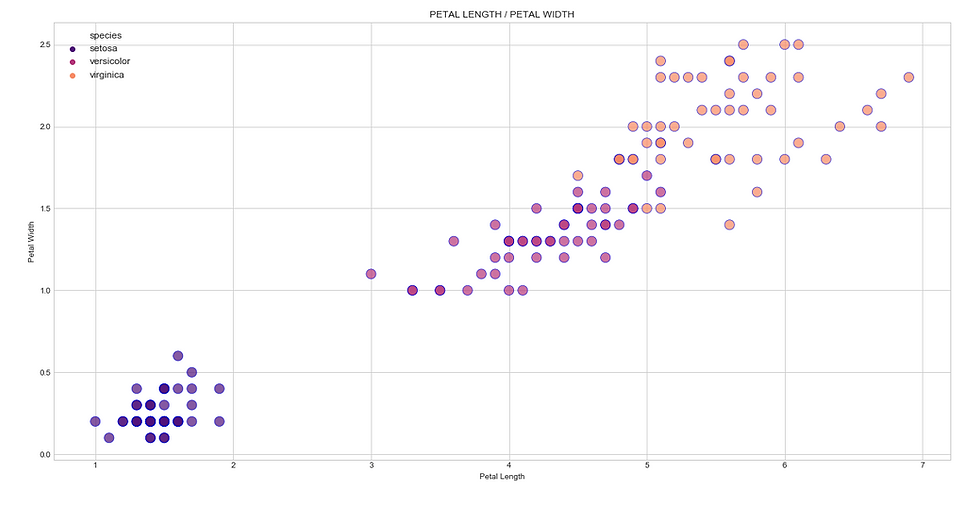
(i) Scatter plot
We are going to create two different scatter plots, one is sepal length against sepal width and the other is petal length against petal width. Let’s do it in python!
Sepal Scatter Python Implementation:
Output:

Petal Scatter Python Implementation:
Output:
(ii) Heatmap
Heatmaps are very useful to find correlations and relations between variables in a data. Heatmaps can be effectively produced using seaborn in python.
Python Implementation:
Output:

(iii) Scatter Matrix
Scatter Matrix is another way to find relations or correlations between variables in a dataset effectively. This plot can also be done using the seaborn library in python.
Python Implementation:
Output:

(iv) Distribution Plot
Distribution plot is used to visualize the frequency of specified values in a dataset. It can be feasibly done in python using the seaborn package.
Python Implementation:
Output:

With this visualization, we are moving on to the next part of coding which is building and training our K-Nearest Neighbor model using scikit-learn in python.
Step-3: Building and Training the model
Firstly, we need to define the ‘X’ variable and a ‘Y’ variable to build our KNN model. Given our dataset, the ‘species’ variable is the one we need to classify and so it can be taken as the ‘Y’ variable or the dependent variable. All the other variables in our dataset can be considered as independent variables or ‘X’ variables. Now, let’s define our X and Y variables in Python!
Python Implementation:
Output:
X variable : [[5.1 3.5 1.4 0.2]
 [4.9 3.  1.4 0.2]
 [4.7 3.2 1.3 0.2]
 [4.6 3.1 1.5 0.2]
 [5.  3.6 1.4 0.2]]
Y variable : ['setosa' 'setosa' 'setosa' 'setosa' 'setosa']
Now, we have to normalize our ‘X’ variable values which can be useful while training our KNN model. To normalize the values, we can make use of the ‘StandardScaler’ function in scikit-learn. Let’s do it in Python!
Python Implementation:
Output:
[[-0.90068117  1.01900435 -1.34022653 -1.3154443 ]
 [-1.14301691 -0.13197948 -1.34022653 -1.3154443 ]
 [-1.38535265  0.32841405 -1.39706395 -1.3154443 ]
 [-1.50652052  0.09821729 -1.2833891  -1.3154443 ]
 [-1.02184904  1.24920112 -1.34022653 -1.3154443 ]]
Now that we have perfect dependent and independent variables. Now, we can proceed with training our KNN model. To train our model, we have to first split our data into a training set and testing set where the training set has the most number of data points. To split our data, we can use the ‘train_test_split’ function provided by scikit-learn in python.
Python Implementation:
Output:
Train set shape : (105, 4) (105,)
Test set shape : (45, 4) (45,)
In the above code, we used ‘the train_test_split’ to split our data into a training set and testing set. Inside the function, we specified our test set should be 30% of the data and the rest is the training set. Finally, we mentioned that there should be no random shuffling of our data while splitting.
We are now ready to create our KNN algorithm. Let’s do it in Python!
Python Implementation:
Output:
KNeighborsClassifier(algorithm='auto',leaf_size=30,metric='minkowski',
                     metric_params=None,n_jobs=None,n_neighbors=3, p=2,
                     weights='uniform')
Firstly, we specified our ‘K’ value to be 3. Next, we defined our algorithm and finally, fitted our train set values into the algorithm. After printing out the algorithm we can see that ‘metric=minkowski’ which is nothing but it states that the method used to calculate the neighbor distance is the Minkowski method. There are also other methods like the Euclidean distance method but it needs to be defined manually.
After finishing training our KNN algorithm, let’s predict the test values by our trained algorithm and evaluate our prediction results using scikit-learn’s evaluation metrics.
Python Implementation:
Output:
Prediction Accuracy Score (%) : 97.78 Using our trained KNN algorithm, we have predicted the test set values. Finally, we used the ‘accuracy_score’ evaluation metric to check the accuracy of our predicted results. In the output, we can see that the results are 97.78% accurate which means our KNN model performed really well for the given iris dataset also, it has the capability to solve real-world classification problems. With that, we have successfully built, trained, and evaluated our KNN model in python.
Final Thoughts!
Now you know the fundamentals of one of the most basic machine learning algorithms. It’s a great place to start when first learning to build models based on different data sets. If you have a dataset with a lot of different points and accurate information, this is a great place to begin exploring machine learning with KNN.
When looking to begin using this algorithm keep these three points in mind:
First, find a dataset that will be easy to work with, ideally one with lots of different points and labeled data.
Second, figure out which language will be easiest for programming to solve the problem (Most recommended is Python).
Third, do your research. It is important to learn the correct practices for using this algorithm so you are finding the most accurate results from your data set.
In conclusion, this is a fundamental machine learning algorithm that is dependable for many reasons like ease of use and quick calculation time. It is a good algorithm to use when beginning to explore the world of machine learning, but it still has room for improvement and modification.
I hope, you find this article useful and don’t worry if you failed to follow any of the coding parts as I’ve provided the full code source for this article.
Happy Machine Learning!
Full code:


Nice Nikhil.. Easy to understand...!! Good Work 👏🏻
Great work on how statistical methods and models are used in Machine Learning. Thank you. Do more!
Got an introduction to KNN & it's use in ML. The simplicity leads to less calculation time and it's capabilities in day to day life. Thanks Nikhil.
Super Nikhil