Algorithmic Trading with Bollinger Bands in Python
- Nikhil Adithyan

- Apr 18, 2021
- 14 min read
Updated: May 1, 2021
An automated way to trade stocks with Bollinger Bands in Python

Disclaimer: This article is strictly for educational purposes and should not be taken as an investment tip.
This is the second article of my algorithmic trading series (view the first article). In the first article, we discussed what algorithmic trading is and learned a stock technical indicator Simple Moving Average (SMA) and how to apply it in python to trade stocks. In this article, we are going to learn a new technical indicator Bollinger Bands and how it can be used to create trading strategies in python. Buckle up your seatbelts for a wonderful ride!
Before that, just a note on what algorithmic trading is. Algorithmic trading is the process of enabling computers to trade stocks under certain conditions or rules. A trade will be performed by the computer automatically when the given condition gets satisfied. Also, these conditions are nothing but trading strategies given to the computers by human traders.
Bollinger Bands
Before jumping on to explore Bollinger Bands, it is essential to know what Simple Moving Average (SMA) is. Simple Moving Average is nothing but the average price of a stock given a specified period of time. Now, Bollinger Bands are trend lines plotted above and below the SMA of the given stock at a specific standard deviation level. To understand Bollinger Bands better, have a look at the following chart that represents the Bollinger Bands of the Tesla stock calculated with SMA 20

Bollinger Bands are great to observe the volatility of a given stock over a period of time. The volatility of a stock is observed to be lower when the space or distance between the upper and lower band is less. Similarly, when the space or distance between the upper and lower band is more, the stock has a higher level of volatility. While observing the chart, you can observe a trend line named ‘MIDDLE BB 20’ which is nothing but SMA 20 of the Tesla stock. The formula to calculate both upper and lowers bands of stock are as follows:
UPPER_BB = STOCK SMA + SMA STANDARD DEVIATION * 2
LOWER_BB = STOCK SMA - SMA STANDARD DEVIATION * 2
Now that we have an understanding of what Bollinger Bands is, so let’s gain some intuitions on the trading strategy we are going to build using Bollinger Bands.
About the trading strategy: We are going to implement a basic trading strategy using the Bollinger Bands indicator which will shoot a buy signal if the stock price of the previous day is greater than the previous day's lower band and the current stock price is lesser than the current day’s lower band. Similarly, if the stock price of the previous day is lesser than the previous day’s upper band and the current stock price is greater than the current day’s upper band, the strategy will reveal a sell signal. Our Bollinger Bands trading strategy can be represented as follows:
IF PREV_STOCK > PREV_LOWERBB & CUR_STOCK < CUR_LOWER_BB => BUY
IF PREV_STOCK < PREV_UPPERBB & CUR_STOCK > CUR_UPPER_BB => SELL
Now that we have an understanding of our Bollinger Bands trading strategy. So, let’s move ahead to build and implement it in python.
Implementation in Python
We are going to implement the trading strategy which we discussed earlier in python to see how well it works in the real world.
Importing packages
Before coding our trading strategy, it is essential to import the required packages into our python environment. The primary packages are going to be Pandas for data manipulation, Matplotlib for plotting purposes, and NumPy for calculations. The additional packages will be Math for mathematical functions, Requests for pulling stock data from API, and Termcolor for font customization.
Python Implementation:
import pandas as pd
import matplotlib.pyplot as plt
import requests
import math
from termcolor import colored as cl
import numpy as np

plt.style.use('fivethirtyeight')
plt.rcParams['figure.figsize'] = (20, 10)
We have imported all the required packages into our python environment. Now let’s extract the historical data of Tesla (TSLA) from IEX Cloud. Before moving on, if you don’t know what is IEX Cloud and how to pull data from it, I highly recommend you to view my article on it (click here to view the article). Let’s pull some data!
Extracting data from IEX Cloud
In this step, we are going to pull the historic data of Tesla using an API provided by IEX Cloud.
Python Implementation:
def get_historic_data(symbol):
    ticker = symbol
    iex_api_key = 'Tsk_30a2677082d54c7b8697675d84baf94b'
    api_url = f'https://sandbox.iexapis.com/stable/stock/{ticker}/chart/max?token={iex_api_key}'
    df = requests.get(api_url).json()

    date = []
    open = []
    high = []
    low = []
    close = []

    for i in range(len(df)):
        date.append(df[i]['date'])
        open.append(df[i]['open'])
        high.append(df[i]['high'])
        low.append(df[i]['low'])
        close.append(df[i]['close'])

    date_df = pd.DataFrame(date).rename(columns = {0:'date'})
    open_df = pd.DataFrame(open).rename(columns = {0:'open'})
    high_df = pd.DataFrame(high).rename(columns = {0:'high'})
    low_df = pd.DataFrame(low).rename(columns = {0:'low'})
    close_df = pd.DataFrame(close).rename(columns = {0:'close'})
    frames = [date_df, open_df, high_df, low_df, close_df]
    df = pd.concat(frames, axis = 1, join = 'inner')
    return df

tsla = get_historic_data('TSLA')
tsla = tsla.set_index('date')
tsla = tsla[tsla.index >= '2020-01-01']
tsla.to_csv('tsla.csv')

tsla = pd.read_csv('tsla.csv').set_index('date')
tsla.index = pd.to_datetime(tsla.index)
tsla.tail()
Output:
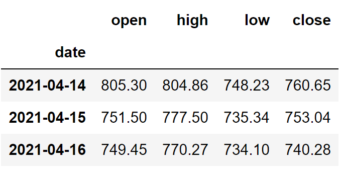
Code Explanation: First we are defining a function named ‘get_historic_data’ that takes a stock’s ticker (‘symbol’) as the parameter. Inside the function, we are storing the API key and the URL into their respective variables, and then using the ‘GET’ method provided by the Request package, we are extracting the data in a JSON format. Next, we are doing some data manipulation tasks to clean and make the data usable. Finally, we are returning the dataframe. After finished defining the function, we are calling it and stored the data into the ‘tsla’ variable. Now, let’s calculate the Bollinger Bands values out of the extracted data.
Bollinger Bands calculation
This is step is further divided into two parts. The first part is to calculate the SMA values and the second is to calculate the Bollinger Bands.
Calculating SMA values: In this part, we are going to calculate the SMA values of Tesla with the number of periods as 20.
Python Implementation:
def sma(data, window):
    sma = data.rolling(window = window).mean()
    return sma

tsla['sma_20'] = sma(tsla['close'], 20)
tsla.tail()
Output:

Code Explanation: Firstly, we are defining a function named ‘sma’ that takes the stock prices (‘data’), and the number of periods (‘window’) as the parameters. Inside the function, we are using the ‘rolling’ function provided by the Pandas package to calculate the SMA for the given number of periods. We are storing the calculated values into the ‘sma’ variable and returned it. Next, we are calling the function and calculated SMA values with the number of periods as 20. Now, let’s calculate the Bollinger Bands.
Calculating Bollinger Bands: In this part, we are going to calculate the Bollinger Bands values of Tesla using the SMA values which we have created earlier.
Python Implementation:
def bb(data, sma, window):
    std = data.rolling(window = window).std()
    upper_bb = sma + std * 2
    lower_bb = sma - std * 2
    return upper_bb, lower_bb

tsla['upper_bb'], tsla['lower_bb'] = bb(tsla['close'], tsla['sma_20'], 20)
tsla.tail()
Output:

Code Explanation: Firstly, we are defining a function named ‘bb’ that takes the stock prices (‘data’), SMA values (‘sma’), and the number of periods as parameters (‘window’). Inside the function, we are using the ‘rolling’ and the ‘std’ function to calculate the standard deviation of the given stock data and stored the calculated standard deviation values into the ‘std’ variable. Next, we are calculating Bollinger Bands values using their respective formulas, and finally, we are returning the calculated values. We are storing the Bollinger Bands values into our ‘tsla’ dataframe using the created ‘bb’ function.
Plotting Bollinger Bands values
In this step, we are going to plot the calculated Bollinger Bands values to make more sense out of them.
Python Implementation:
tsla['close'].plot(label = 'CLOSE PRICES', color = 'skyblue')
tsla['upper_bb'].plot(label = 'UPPER BB 20', linestyle = '--', linewidth = 1, color = 'black')
tsla['sma_20'].plot(label = 'MIDDLE BB 20', linestyle = '--', linewidth = 1.2, color = 'grey')
tsla['lower_bb'].plot(label = 'LOWER BB 20', linestyle = '--', linewidth = 1, color = 'black')
plt.legend(loc = 'upper left')
plt.title('TSLA BOLLINGER BANDS')
plt.show()
Output:

Code Explanation: Using the ‘plot’ function provided by the Matplotlib package, we have plotted the Bollinger Band values along with the ‘close’ prices of Tesla. Now let’s observe the graph. The light blue line represents the ‘close’ prices of Tesla, and the black dotted line represents the lower and upper bands. Similarly, the grey dotted line represents the middle band or the SMA 20 values of Tesla. We can also observe that the spaces between the upper and lower bands are becoming narrow or wider at different times representing the volatility of the stock.
WIDER SPACE == HIGH VOLATILITY
NARROW SPACE == LOW VOLATILITY
Creating the Trading Strategy
In this step, we are going to implement the discussed Bollinger Bands trading strategy in python.
Python Implementation:
def implement_bb_strategy(data, lower_bb, upper_bb):
    buy_price = []
    sell_price = []
    bb_signal = []
    signal = 0

    for i in range(len(data)):
        if data[i-1] > lower_bb[i-1] and data[i] < lower_bb[i]:
            if signal != 1:
                buy_price.append(data[i])
                sell_price.append(np.nan)
                signal = 1
                bb_signal.append(signal)
            else:
                buy_price.append(np.nan)
                sell_price.append(np.nan)
                bb_signal.append(0)
        elif data[i-1] < upper_bb[i-1] and data[i] > upper_bb[i]:
            if signal != -1:
                buy_price.append(np.nan)
                sell_price.append(data[i])
                signal = -1
                bb_signal.append(signal)
            else:
                buy_price.append(np.nan)
                sell_price.append(np.nan)
                bb_signal.append(0)
        else:
            buy_price.append(np.nan)
            sell_price.append(np.nan)
            bb_signal.append(0)

    return buy_price, sell_price, bb_signal

buy_price, sell_price, bb_signal = implement_bb_strategy(tsla['close'], tsla['lower_bb'], tsla['upper_bb'])
Code Explanation: First, we are defining a function named ‘implement_bb_strategy’ which takes the stock prices (‘data’), lower band values (‘lower_bb’), and upper band values (‘upper_bb’) as parameters.
Inside the function, we are creating three empty lists (buy_price, sell_price, and bb_signal) in which the values will be appended while creating the trading strategy.
After that, we are implementing the trading strategy through a for-loop. Inside the for-loop, we are passing certain conditions, and if the conditions are satisfied, the respective values will be appended to the empty lists. If the condition to buy the stock gets satisfied, the buying price will be appended to the ‘buy_price’ list, and the signal value will be appended as 1 representing to buy the stock. Similarly, if the condition to sell the stock gets satisfied, the selling price will be appended to the ‘sell_price’ list, and the signal value will be appended as -1 representing to sell the stock.
Finally, we are returning the lists appended with values. Then, we are calling the created function and stored the values into their respective variables. The list doesn’t make any sense unless we plot the values. So, let’s plot the values of the created trading lists.
Plotting the Trading lists
In this step, we are going to plot the created trading lists to make sense out of them.
Python Implementation:
tsla['close'].plot(label = 'CLOSE PRICES', alpha = 0.3)
tsla['upper_bb'].plot(label = 'UPPER BB', linestyle = '--', linewidth = 1, color = 'black')
tsla['sma_20'].plot(label = 'MIDDLE BB', linestyle = '--', linewidth = 1.2, color = 'grey')
tsla['lower_bb'].plot(label = 'LOWER BB', linestyle = '--', linewidth = 1, color = 'black')
plt.scatter(tsla.index, buy_price, marker = '^', color = 'green', label = 'BUY', s = 200)
plt.scatter(tsla.index, sell_price, marker = 'v', color = 'red', label = 'SELL', s = 200)
plt.title('TSLA BB STRATEGY TRADING SIGNALS')
plt.legend(loc = 'upper left')
plt.show()
Output:

Code Explanation: We are plotting the Bollinger Bands values along with the buy and sell signals generated by the trading strategy. We can observe that whenever the stock’s close price (light blue line) below the lower band (lower black dotted line), a buy signal is plotted in green color, similarly, whenever the stock’s close price crosses above the upper band (upper black dotted line), a sell signal is plotted in red color.
Now, using the trading signals, let’s create our position on the stock.
Creating our Position
In this step, we are going to create a list that indicates 1 if we hold the stock or 0 if we don’t own or hold the stock.
Python Implementation:
position = []
for i in range(len(bb_signal)):
    if bb_signal[i] > 1:
        position.append(0)
    else:
        position.append(1)

for i in range(len(tsla['close'])):
    if bb_signal[i] == 1:
        position[i] = 1
    elif bb_signal[i] == -1:
        position[i] = 0
    else:
        position[i] = position[i-1]

upper_bb = tsla['upper_bb']
lower_bb = tsla['lower_bb']
close_price = tsla['close']
bb_signal = pd.DataFrame(bb_signal).rename(columns = {0:'bb_signal'}).set_index(tsla.index)
position = pd.DataFrame(position).rename(columns = {0:'bb_position'}).set_index(tsla.index)

frames = [close_price, upper_bb, lower_bb, bb_signal, position]
strategy = pd.concat(frames, join = 'inner', axis = 1)
strategy = strategy.reset_index().drop('date', axis = 1)

strategy.tail(7)
Output:

Code Explanation: First, we are creating an empty list named ‘position’. We are passing two for-loops, one is to generate values for the ‘position’ list to just match the length of the ‘signal’ list. The other for-loop is the one we are using to generate actual position values. Inside the second for-loop, we are iterating over the values of the ‘signal’ list, and the values of the ‘position’ list get appended concerning which condition gets satisfied. The value of the position remains 1 if we hold the stock or remains 0 if we sold or don’t own the stock. Finally, we are doing some data manipulations to combine all the created lists into one dataframe.
From the output being shown, we can see that from row 318–320, our position in the stock has remained 1 (since there isn’t any change in the Bollinger Bands signal) but our position suddenly turned to 0 as we sold the stock when the Bollinger Bands trading signal represents a sell signal (-1). Now it’s time to do implement some backtesting process!
Backtesting
Before moving on, it is essential to know what backtesting is. Backtesting is the process of seeing how well our trading strategy has performed on the given stock data. In our case, we are going to implement a backtesting process for our Bollinger Bands trading strategy over the Tesla stock data.
Python Implementation:
tsla_ret = pd.DataFrame(np.diff(tsla['close'])).rename(columns = {0:'returns'})
bb_strategy_ret = []

for i in range(len(tsla_ret)):
    try:
        returns = tsla_ret['returns'][i]*strategy['bb_position'][i]
        bb_strategy_ret.append(returns)
    except:
        pass

bb_strategy_ret_df = pd.DataFrame(bb_strategy_ret).rename(columns = {0:'bb_returns'})

investment_value = 100000
number_of_stocks = math.floor(investment_value/tsla['close'][-1])
bb_investment_ret = []

for i in range(len(bb_strategy_ret_df['bb_returns'])):
    returns = number_of_stocks*bb_strategy_ret_df['bb_returns'][i]
    bb_investment_ret.append(returns)

bb_investment_ret_df = pd.DataFrame(bb_investment_ret).rename(columns = {0:'investment_returns'})
total_investment_ret = round(sum(bb_investment_ret_df['investment_returns']), 2)
profit_percentage = math.floor((total_investment_ret/investment_value)*100)
print(cl('Profit gained from the BB strategy by investing $100k in TSLA : {}'.format(total_investment_ret), attrs = ['bold']))
print(cl('Profit percentage of the BB strategy : {}%'.format(profit_percentage), attrs = ['bold']))
Output:
Profit gained from the BB strategy by investing $100k in TSLA: 18426.42
Profit percentage of the BB strategy: 18%
Code Explanation: First, we are calculating the returns of the Tesla stock using the ‘diff’ function provided by the NumPy package and we have stored it as a dataframe into the ‘tsla_ret’ variable. Next, we are passing a for-loop to iterate over the values of the ‘tsla_ret’ variable to calculate the returns we gained from our Bollinger Bands trading strategy, and these returns values are appended to the ‘bb_strategy_ret’ list. Next, we are converting the ‘bb_strategy_ret’ list into a dataframe and stored it into the ‘bb_strategy_ret_df’ variable.
Next comes the backtesting process. We are going to backtest our strategy by investing a hundred thousand USD into our trading strategy. So first, we are storing the amount of investment into the ‘investment_value’ variable. After that, we are calculating the number of Tesla stocks we can buy using the investment amount. You can notice that I’ve used the ‘floor’ function provided by the Math package because, while dividing the investment amount by the closing price of Tesla stock, it spits out an output with decimal numbers. The number of stocks should be an integer but not a decimal number. Using the ‘floor’ function, we can cut out the decimals. Remember that the ‘floor’ function is way more complex than the ‘round’ function. Then, we are passing a for-loop to find the investment returns followed by some data manipulations tasks.
Finally, we are printing the total return we got by investing a hundred thousand into our trading strategy and it is revealed that we have made an approximate profit of eighteen thousand and five hundred USD in one year. That’s not bad! Now, let’s compare our returns with SPY ETF (an ETF designed to track the S&P 500 stock market index) returns.
SPY ETF Comparison
This step is optional but it is highly recommended as we can get an idea of how well our trading strategy performs against a benchmark (SPY ETF). In this step, we are going to extract the data of the SPY ETF using the ‘get_historic_data’ function we created and compare the returns we get from the SPY ETF with our Bollinger Bands strategy returns on Tesla.
Python Implementation:
def get_benchmark(stock_prices, start_date, investment_value):
    spy = get_historic_data('SPY')
    spy = spy.set_index('date')
    spy = spy[spy.index >= start_date]['close']
    benchmark = pd.DataFrame(np.diff(spy)).rename(columns = {0:'benchmark_returns'})

    investment_value = investment_value
    number_of_stocks = math.floor(investment_value/stock_prices[-1])
    benchmark_investment_ret = []

    for i in range(len(benchmark['benchmark_returns'])):
        returns = number_of_stocks*benchmark['benchmark_returns'][i]
        benchmark_investment_ret.append(returns)

    benchmark_investment_ret_df = pd.DataFrame(benchmark_investment_ret).rename(columns = {0:'investment_returns'})
    return benchmark_investment_ret_df

benchmark = get_benchmark(tsla['close'], '2020-01-01', 100000)

investment_value = 100000
total_benchmark_investment_ret = round(sum(benchmark['investment_returns']), 2)
benchmark_profit_percentage = math.floor((total_benchmark_investment_ret/investment_value)*100)
print(cl('Benchmark profit by investing $100k : {}'.format(total_benchmark_investment_ret), attrs = ['bold']))
print(cl('Benchmark Profit percentage : {}%'.format(benchmark_profit_percentage), attrs = ['bold']))
print(cl('BB Strategy profit is {}% higher than the Benchmark Profit'.format(profit_percentage - benchmark_profit_percentage), attrs = ['bold']))
Output:
Benchmark profit by investing $100k : 13270.5
Benchmark Profit percentage : 13%
BB Strategy profit is 5% higher than the Benchmark Profit
Code Explanation: The code used in this step is almost similar to the one used in the previous backtesting step but, instead of investing in Tesla, we are investing in SPY ETF by not implementing any trading strategies. From the output, we can see that our Bollinger Bands trading strategy has outperformed the SPY ETF by 5%. That’s great!
Conclusion
In this article, we learned a new stock technical indicator which is Bollinger Bands and the ways to implement and backtest a Bollinger Bands trading strategy in python. The trading strategy we implemented in this article is a basic one but, there are a lot of trading strategies based on Bollinger Bands to be applied. It is believed that Bollinger Bands are not that good for algorithmic trading but they can be effective with the right trading strategy. There are also several ways to improve this article which are:
Picking stocks: In this article, we randomly chose Tesla but, it isn’t a wise decision to make in the real world. Instead, Machine Learning algorithms can be applied to pick the right tradable stocks. This step is a really important part of algorithmic trading in the real world and in case, the stocks are randomly chosen, the results would be catastrophic.
Strategy improvement: As I said before, the trading strategy we used in this article is an elementary-level strategy and it would not perform exceptionally when applied in the real world. So, it is highly recommended to discover more Bollinger Bands strategies and implement them in python.
That’s it! If you forgot to follow any of the coding parts, don’t worry! I’ve provided the full source code of this article at the end. Hope you got some idea on Bollinger Bands out of this article.
Full code:
import pandas as pd
import matplotlib.pyplot as plt
import requests
import math
from termcolor import colored as cl
import numpy as np

plt.style.use('fivethirtyeight')
plt.rcParams['figure.figsize'] = (20, 10)

def get_historic_data(symbol):
    ticker = symbol
    iex_api_key = 'Tsk_30a2677082d54c7b8697675d84baf94b'
    api_url = f'https://sandbox.iexapis.com/stable/stock/{ticker}/chart/max?token={iex_api_key}'
    df = requests.get(api_url).json()

    date = []
    open = []
    high = []
    low = []
    close = []

    for i in range(len(df)):
        date.append(df[i]['date'])
        open.append(df[i]['open'])
        high.append(df[i]['high'])
        low.append(df[i]['low'])
        close.append(df[i]['close'])

    date_df = pd.DataFrame(date).rename(columns = {0:'date'})
    open_df = pd.DataFrame(open).rename(columns = {0:'open'})
    high_df = pd.DataFrame(high).rename(columns = {0:'high'})
    low_df = pd.DataFrame(low).rename(columns = {0:'low'})
    close_df = pd.DataFrame(close).rename(columns = {0:'close'})
    frames = [date_df, open_df, high_df, low_df, close_df]
    df = pd.concat(frames, axis = 1, join = 'inner')
    return df

tsla = pd.read_csv('tsla.csv').set_index('date')
tsla.index = pd.to_datetime(tsla.index)
print(tsla.tail())

plt.plot(tsla.index, tsla['close'])
plt.xlabel('Date')
plt.ylabel('Closing Prices')
plt.title('TSLA Stock Prices 2020-2021')
plt.show()

def sma(data, window):
    sma = data.rolling(window = window).mean()
    return sma

tsla['sma_20'] = sma(tsla['close'], 20)
print(tsla.tail())

tsla['close'].plot(label = 'CLOSE', alpha = 0.6)
tsla['sma_20'].plot(label = 'SMA 20', linewidth = 2)
plt.xlabel('Date')
plt.ylabel('Closing Prices')
plt.legend(loc = 'upper left')
plt.show()

def bb(data, sma, window):
    std = data.rolling(window = window).std()
    upper_bb = sma + std * 2
    lower_bb = sma - std * 2
    return upper_bb, lower_bb

tsla['upper_bb'], tsla['lower_bb'] = bb(tsla['close'], tsla['sma_20'], 20)
print(tsla.tail())

tsla['close'].plot(label = 'CLOSE PRICES', color = 'skyblue')
tsla['upper_bb'].plot(label = 'UPPER BB 20', linestyle = '--', linewidth = 1, color = 'black')
tsla['sma_20'].plot(label = 'MIDDLE BB 20', linestyle = '--', linewidth = 1.2, color = 'grey')
tsla['lower_bb'].plot(label = 'LOWER BB 20', linestyle = '--', linewidth = 1, color = 'black')
plt.legend(loc = 'upper left')
plt.title('TSLA BOLLINGER BANDS')
plt.show()

def implement_bb_strategy(data, lower_bb, upper_bb):
    buy_price = []
    sell_price = []
    bb_signal = []
    signal = 0

    for i in range(len(data)):
        if data[i-1] > lower_bb[i-1] and data[i] < lower_bb[i]:
            if signal != 1:
                buy_price.append(data[i])
                sell_price.append(np.nan)
                signal = 1
                bb_signal.append(signal)
            else:
                buy_price.append(np.nan)
                sell_price.append(np.nan)
                bb_signal.append(0)
        elif data[i-1] < upper_bb[i-1] and data[i] > upper_bb[i]:
            if signal != -1:
                buy_price.append(np.nan)
                sell_price.append(data[i])
                signal = -1
                bb_signal.append(signal)
            else:
                buy_price.append(np.nan)
                sell_price.append(np.nan)
                bb_signal.append(0)
        else:
            buy_price.append(np.nan)
            sell_price.append(np.nan)
            bb_signal.append(0)

    return buy_price, sell_price, bb_signal

buy_price, sell_price, bb_signal = implement_bb_strategy(tsla['close'], tsla['lower_bb'], tsla['upper_bb'])

tsla['close'].plot(label = 'CLOSE PRICES', alpha = 0.3)
tsla['upper_bb'].plot(label = 'UPPER BB', linestyle = '--', linewidth = 1, color = 'black')
tsla['sma_20'].plot(label = 'MIDDLE BB', linestyle = '--', linewidth = 1.2, color = 'grey')
tsla['lower_bb'].plot(label = 'LOWER BB', linestyle = '--', linewidth = 1, color = 'black')
plt.scatter(tsla.index, buy_price, marker = '^', color = 'green', label = 'BUY', s = 200)
plt.scatter(tsla.index, sell_price, marker = 'v', color = 'red', label = 'SELL', s = 200)
plt.title('TSLA BB STRATEGY TRADING SIGNALS')
plt.legend(loc = 'upper left')
plt.show()

position = []
for i in range(len(bb_signal)):
    if bb_signal[i] > 1:
        position.append(0)
    else:
        position.append(1)

for i in range(len(tsla['close'])):
    if bb_signal[i] == 1:
        position[i] = 1
    elif bb_signal[i] == -1:
        position[i] = 0
    else:
        position[i] = position[i-1]

upper_bb = tsla['upper_bb']
lower_bb = tsla['lower_bb']
close_price = tsla['close']
bb_signal = pd.DataFrame(bb_signal).rename(columns = {0:'bb_signal'}).set_index(tsla.index)
position = pd.DataFrame(position).rename(columns = {0:'bb_position'}).set_index(tsla.index)

frames = [close_price, upper_bb, lower_bb, bb_signal, position]
strategy = pd.concat(frames, join = 'inner', axis = 1)
strategy = strategy.reset_index().drop('date', axis = 1)

print(strategy.tail(7))

tsla_ret = pd.DataFrame(np.diff(tsla['close'])).rename(columns = {0:'returns'})
bb_strategy_ret = []

for i in range(len(tsla_ret)):
    try:
        returns = tsla_ret['returns'][i]*strategy['bb_position'][i]
        bb_strategy_ret.append(returns)
    except:
        pass

bb_strategy_ret_df = pd.DataFrame(bb_strategy_ret).rename(columns = {0:'bb_returns'})

investment_value = 100000
number_of_stocks = math.floor(investment_value/tsla['close'][-1])
bb_investment_ret = []

for i in range(len(bb_strategy_ret_df['bb_returns'])):
    returns = number_of_stocks*bb_strategy_ret_df['bb_returns'][i]
    bb_investment_ret.append(returns)

bb_investment_ret_df = pd.DataFrame(bb_investment_ret).rename(columns = {0:'investment_returns'})
total_investment_ret = round(sum(bb_investment_ret_df['investment_returns']), 2)
profit_percentage = math.floor((total_investment_ret/investment_value)*100)
print(cl('Profit gained from the BB strategy by investing $100k in TSLA : {}'.format(total_investment_ret), attrs = ['bold']))
print(cl('Profit percentage of the BB strategy : {}%'.format(profit_percentage), attrs = ['bold']))

def get_benchmark(stock_prices, start_date, investment_value):
    spy = get_historic_data('SPY')
    spy = spy.set_index('date')
    spy = spy[spy.index >= start_date]['close']
    benchmark = pd.DataFrame(np.diff(spy)).rename(columns = {0:'benchmark_returns'})

    investment_value = investment_value
    number_of_stocks = math.floor(investment_value/stock_prices[-1])
    benchmark_investment_ret = []

    for i in range(len(benchmark['benchmark_returns'])):
        returns = number_of_stocks*benchmark['benchmark_returns'][i]
        benchmark_investment_ret.append(returns)

    benchmark_investment_ret_df = pd.DataFrame(benchmark_investment_ret).rename(columns = {0:'investment_returns'})
    return benchmark_investment_ret_df

benchmark = get_benchmark(tsla['close'], '2020-01-01', 100000)

investment_value = 100000
total_benchmark_investment_ret = round(sum(benchmark['investment_returns']), 2)
benchmark_profit_percentage = math.floor((total_benchmark_investment_ret/investment_value)*100)
print(cl('Benchmark profit by investing $100k : {}'.format(total_benchmark_investment_ret), attrs = ['bold']))
print(cl('Benchmark Profit percentage : {}%'.format(benchmark_profit_percentage), attrs = ['bold']))
print(cl('BB Strategy profit is {}% higher than the Benchmark Profit'.format(profit_percentage - benchmark_profit_percentage), attrs = ['bold']))


Though too much technical issues are involved, Nikil has done a good job to make it easy to understand
A glimpse of next gen trading. Thanks Nikhil
Good One but highly technical Nikhil