An Algo Trading Strategy which made +8,371%: A Python Case Study
- Nikhil Adithyan

- Jan 3, 2024
- 6 min read
Backtesting of a simple breakout trading strategy with APIs and Python

Introduction
There is literally no point in going after traditional algo trading strategies like SMA crossover or RSI threshold breakout strategy as it has proven to be obsolete given their simplistic nature and more importantly, the massive volume of participants who are trying to implement them in the market.
So instead of embracing those strategies, it’s time to try something new. In this article, we’ll be using Python and Benzinga’s APIs to construct and backtest a new trading strategy that will help us beat the market.
With that being said, let’s dive into the article!
The Trading Strategy
Before moving to the coding part, it’s essential to have a good background on the strategy we’re going to build in this article. Our trading strategy follows the principle of simplicity yet a very effective breakout strategy.
We enter the market if: the stock’s current high exceeds the 50-week high
We exit the market if: the stock’s current low sinks below the 40-week low
We’ll be using the Donchian Channel indicator in order to keep track of the 50-week high and the 40-week low. This strategy is a weekly trading system, so, we’ll be backtesting it on the weekly timeframe.
And, there you go! This is the strategy we’re going to backtest in this article. As simple as it is, right?! Now, let’s move on to the coding part of the article.
Importing Packages
In this article, we are going to use four primary packages which are pandas, requests, pandas_ta and matplotlib, and the secondary/optional packages include termcolor and math. The following code will import all the mentioned packages into our Python environment:
# IMPORTING PACKAGES

import pandas as pd
import requests
import pandas_ta as ta
import matplotlib.pyplot as plt
from termcolor import colored as cl
import math

plt.rcParams['figure.figsize'] = (20,10)
plt.style.use('fivethirtyeight')
If you haven’t installed any of the imported packages, make sure to do so using the pip command in your terminal.
Extracting Historical Data
We are going to backtest our breakout strategy on Apple’s stock. So in order to obtain the historical stock data of Apple, we are going to use Benzinga’s Historical Bar Data API endpoint. The following Python code uses the endpoint to extract Apple’s stock data from 1993:
# EXTRACTING HISTORICAL DATA

def get_historical_data(symbol, start_date, interval):
    url = "https://api.benzinga.com/api/v2/bars"
    querystring = {"token":"YOUR API KEY","symbols":f"{symbol}","from":f"{start_date}","interval":f"{interval}"}

    hist_json = requests.get(url, params = querystring).json()
    df = pd.DataFrame(hist_json[0]['candles'])

    return df

aapl = get_historical_data('AAPL', '1993-01-01', '1W')
aapl.tail()
In the above code, we are defining a function named get_historical_data which takes the stock symbol, the starting date of the data, and the interval between the data points.
Inside the function, we are storing the API URL and the query strings into their respective variables. Make sure to replace YOUR API KEY with secret Benzinga API key which you can obtain after creating an account with them. Then, we are making an API call to obtain the data and converting the JSON response into a Pandas dataframe which we are returning at the end.
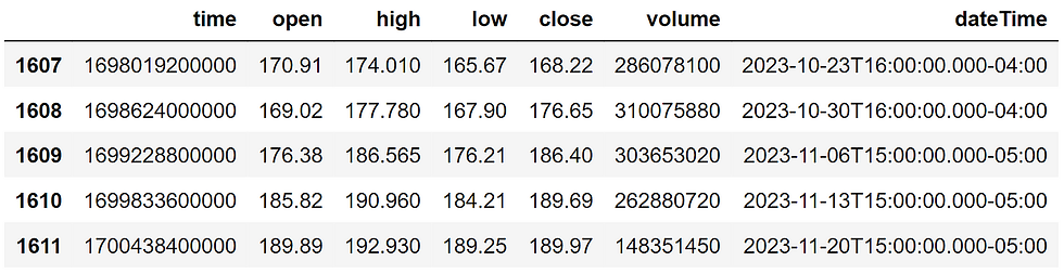
Using the defined function, we are extracting Apple’s historical stock data from 1993 on a weekly timeframe. This is the end output:
Awesome, now let’s move on to calculating the Donchian Channel indicator for the extracted historical data of Apple.
Donchian Channel Calculation
If we dive deep into the mathematics of the indicator, it will demand a separate article on its own for the explanations. So here's a general overview of the indicator. Basically, the Donchian Channel reveals the highest high and the lowest low of a stock over a specified period of time.
The following code uses pandas_ta for the calculation of the indicator:
# CALCULATING DONCHIAN CHANNEL

aapl[['dcl', 'dcm', 'dcu']] = aapl.ta.donchian(lower_length = 40, upper_length = 50)
aapl = aapl.dropna().drop('time', axis = 1).rename(columns = {'dateTime':'date'})
aapl = aapl.set_index('date')
aapl.index = pd.to_datetime(aapl.index)

aapl.tail()
In the first line, we are using the donchian function provided by pandas_ta to calculate the indicator. The function takes two parameters: the lower length and the upper length which are the lookback periods for the lowest low and highest high respectively. We are mentioning the lower and upper lengths as 40 and 50 respectively since our strategy demands 40-week low and 50-week high.
After the calculation, we are performing some data manipulation tasks to clean and format the data. This is the final dataframe:
To get a better view of the Donchian Channel indicator, let’s plot the calculated values using the Matplotlib library:
# PLOTTING DONCHIAN CHANNEL

plt.plot(aapl[-300:].close, label = 'CLOSE')
plt.plot(aapl[-300:].dcl, color = 'black', linestyle = '--', alpha = 0.3)
plt.plot(aapl[-300:].dcm, color = 'orange', label = 'DCM')
plt.plot(aapl[-300:].dcu, color = 'black', linestyle = '--', alpha = 0.3, label = 'DCU,DCL')
plt.legend()
plt.title('AAPL DONCHIAN CHANNELS 50')
plt.xlabel('Date')
plt.ylabel('Close')
There is nothing much going on with this code. We are utilizing all the essential functions provided by matplotlib to create the visualization and this is the final chart:
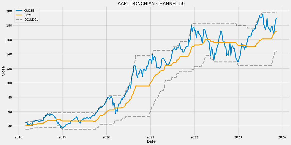
From the plot it can be observed that there are three important components in the Donchian Channel Indicator:
Upper Band: The upper band reveals the highest high of the stock over a specified period of time.
Lower Band: Basically the opposite of the upper band, it shows the lowest low of the stock over a specified period of time.
Middle Band: This component is a little different. It shows the average between the upper band and the lower band.
Donchian Channel is one of the most widely used indicators for observing breakouts happening in stock price movements and that's one of the core reasons for using it in this article.
Backtesting the Strategy
We have arrived at one of the most important steps in this article which is backtesting our breakout strategy. We are going to follow a very basic and straightforward system of backtesting for the sake of simplicity. The following code backtests the strategy and reveals its results:
# BACKTESTING THE STRATEGY

def implement_strategy(aapl, investment):

    in_position = False
    equity = investment

    for i in range(3, len(aapl)):
        if aapl['high'][i] == aapl['dcu'][i] and in_position == False:
            no_of_shares = math.floor(equity/aapl.close[i])
            equity -= (no_of_shares * aapl.close[i])
            in_position = True
            print(cl('BUY: ', color = 'green', attrs = ['bold']), f'{no_of_shares} Shares are bought at ${aapl.close[i]} on {str(aapl.index[i])[:10]}')
        elif aapl['low'][i] == aapl['dcl'][i] and in_position == True:
            equity += (no_of_shares * aapl.close[i])
            in_position = False
            print(cl('SELL: ', color = 'red', attrs = ['bold']), f'{no_of_shares} Shares are bought at ${aapl.close[i]} on {str(aapl.index[i])[:10]}')
    if in_position == True:
        equity += (no_of_shares * aapl.close[i])
        print(cl(f'\nClosing position at {aapl.close[i]} on {str(aapl.index[i])[:10]}', attrs = ['bold']))
        in_position = False

    earning = round(equity - investment, 2)
    roi = round(earning / investment * 100, 2)
    print(cl(f'EARNING: ${earning} ; ROI: {roi}%', attrs = ['bold']))

implement_strategy(aapl, 100000)
I’m not going to dive deep into the dynamics of this code as it will take some time to explain it. Basically, the program executes the trades based on the conditions that are satisfied. It enters the market when our entry condition is satisfied and exits when the exit condition is satisfied. These are trades executed by our program followed by the backtesting results:
As I’ve claimed in the title of the article, our strategy has made an ROI of 8371% which is humongous. But it’s time to see if our strategy has really outperformed the market.
SPY ETF Comparison
Drawing a comparison between the backtesting results of our strategy and the buy/hold returns of the SPY ETF helps us get a true sense of our strategy’s performance. The following code calculates the returns of SPY ETF over the years:
spy = get_historical_data('SPY', '1993-01-01', '1W')
spy_ret = round(((spy.close.iloc[-1] - spy.close.iloc[0])/spy.close.iloc[0])*100)

print(cl('SPY ETF buy/hold return:', attrs = ['bold']), f'{spy_ret}%')
In the above code, we are first extracting the historical data of SPY with the same specifications we used for AAPL. Then we are calculating the returns percentage of the index using a simple formula and this is the result:
The return of the index is 936% which is actually pretty good but when compared to that of our strategy, there is a vast difference. Our strategy has outperformed the benchmark substantially and that’s great news!
Closing Notes
In this article, we went through an extensive process of coding to backtest a simple yet very effective breakout strategy. And as expected, the results of the strategy were amazing. We started off with extracting the historical data of Apple using Benzinga’s API, then slowly explored the Donchian Channel, and finally proceeded to backtest the strategy and compare the results with SPY ETF.
There are still a lot of aspects that can be improved. The backtesting system can be even more complex and realistic with the addition of brokerage commission and slippage. A proper risk management system must be in place, especially in the case of algo trading. Like these, there are many aspects to be improved which I’m leaving to you guys to explore.
With that being said, you’ve reached the end of the article. Before ending the article, I would like to give a shoutout to Benzinga for creating such a great library of APIs which includes institutional-grade market news & data APIs and I would suggest you guys check it out too. Hope you learned something new and useful today. Thank you for your time.


The year 2024 offers a number of intriguing possibilities for anyone interested in exploring the realm of Australian crypto casinos. Leading the charge are sites like Rakebit.com, which provides over seven thousand games, allows for immediate payouts, and offers a substantial welcome bonus of one hundred free spins on a twenty dollar T deposit. The continued existence of crypto casinos is confirmed by their support for several cryptocurrencies, including as Bitcoin, Ethereum, Tron, and even Ton. Players are drawn to Rakebit because of the additional cashback offer of up to 25%. Also, you should check out Justbit.io and Metaspins.com if you're looking for a dependable, user-friendly platform with fast payments and a huge library of games. A first-rate gaming experience…
How can we use the same for symbols of NSEINDIA. Com
Why are we comparing it to SPY and not buying and holding apple stock from 93?