Increasing Stock Returns by Combining Williams %R and MACD in Python
- Nikhil Adithyan

- Aug 1, 2021
- 19 min read
Updated: Aug 5, 2021
A detailed case study on using python to combine two technical indicators and create a killer trading strategy

Technical indicators are the new-common in the trading arena and it is worth the time to study those. Though it has greater potential in analyzing the market, one should definitely consider its drawbacks too. There aren’t many but one notable snag is its nature of revealing false signals which can lead to catastrophic results when followed. It is tough to avoid such signals but are not inevitable and one of the best ways of doing so is to combine two technical indicators where one indicator acts as a filter that classifies the authentic signals from the false ones. That’s exactly what we’re going to do today.
In this article, we are going to combine two powerful technical indicators which are Williams %R and Moving Average Convergence/Divergence (MACD) to create a killer trading strategy that eradicates false trading signals as much as possible and substantially improve the investment returns. Without further ado, let’s dive into the article.
Williams %R
Founded by Larry Williams, the Williams %R is a momentum indicator whose values oscillate between 0 to -100. This indicator is most similar to the Stochastic Oscillator but differs in its calculation. Traders use this indicator to spot potential entry and exit points for trades by constructing two levels of overbought and oversold. Before moving a word on overbought and oversold levels: A stock is said to be overbought when the market’s trend seems to be extremely bullish and bound to consolidate. Similarly, a stock reaches an oversold region when the market’s trend seems to be extremely bearish and has the tendency to bounce. The traditional threshold for overbought and oversold levels are 20 and 80 respectively but there aren’t any prohibitions in taking other values too.
In order to calculate the values of Williams %R with the traditional setting of 14 as the lookback period, first, the highest high and the lowest low for each period over a fourteen-day timeframe is determined. Then, the two differences are taken: The closing price from the highest high, and the lowest low from the highest high. Finally, the first difference is divided by the second difference and multiple by -100 to obtain the values of Williams %R. The calculation can be mathematically represented as follows:
W%R 14 = [ H.HIGH - C.PRICE ] / [ L.LOW - C.PRICE ] * ( - 100 )

where,
W%R 14 = 14-day Williams %R of the stock
H.HIGH = 14-day Highest High of the stock
L.LOW = 14-day Lowest Low of the stock
C.PRICE = Closing price of the stock
The underlying idea of this indicator is that the stock will keep reaching new highs when it is a strong uptrend and similarly, the stock will reach new lows when it follows a sturdy downtrend. Now, let’s analyze a chart of Williams %R to build a strong understanding of the indicator.

The above chart is divided into two panels: The upper panel with the closing price of Apple’s stock data and the lower panel with the values of Apple’s14-day readings of Williams %R. Now, the chart can be utilized in two ways. The first way is using the chart as a tool to identify overbought and oversold states of the market. You could observe that there are two horizontal grey lines plotted above and below the market which is nothing but the overbought and oversold levels plotted at a threshold of -20 and -80 respectively. You can consider that the market is in the state of overbought if the Williams %R has a reading of above the upper line or the overbought line. Similarly, you can assume that the market is in the state of oversold if the Williams %R has a reading of below the lower line or the oversold line.
The second way of using Williams %R is to identify false momentum in the market. During a sturdy uptrend, the readings of Williams %R tend to reach above -20 frequently. If the indicator falls and struggles to reach above -20 before the next fall, indicates that the market’s momentum is not authentic and is possible to follow a tremendous downtrend. Likewise, during a healthy downtrend, the readings of Williams %R are bound to go below -80 frequently. If the indicator rises and fails to reach -80 before the next rise, reveals that the market is going to follow a positive trend.
Since Williams %R is a directional indicator (an indicator whose movement is directly proportional to that of the actual market), traders also use this indicator to find and confirm strong uptrends or downtrends in a market and trade along with it. Some indicators are not of much use while utilized for identifying or confirming market trends as they might be lagging in nature (an indicator that takes into account the historical data points to determine the current reading) but Williams %R is an effective one because it is a leading indicator (an indicator that takes into account the previous data points to predict the future movements).
MACD
Before moving on to MACD, it is essential to know what Exponential Moving Average (EMA) means. EMA is a type of Moving Average (MA) that automatically allocates greater weighting (nothing but importance) to the most recent data point and lesser weighting to data points in the distant past. For example, a question paper would consist of 10% of one mark questions, 40% of three mark questions, and 50% of long answer questions. From this example, you can observe that we are assigning unique weights to each section of the question paper based on the importance level (probably long answer questions are given more importance than the one mark questions).
Now, MACD is a trend-following leading indicator that is calculated by subtracting two Exponential Moving Averages (one with longer and the other shorter periods). There are three notable components in a MACD indicator.
MACD Line: This line is the difference between two given Exponential Moving Averages. To calculate the MACD line, one EMA with a longer period known as slow length and another EMA with a shorter period known as fast length is calculated. The most popular length of the fast and slow is 12, 26 respectively. The final MACD line values can be arrived at by subtracting the slow length EMA from the fast length EMA. The formula to calculate the MACD line can be represented as follows:
MACD LINE = FAST LENGTH EMA - SLOW LENGTH EMA
Signal Line: This line is the Exponential Moving Average of the MACD line itself for a given period of time. The most popular period to calculate the Signal line is 9. As we are averaging out the MACD line itself, the Signal line will be smoother than the MACD line.
Histogram: As the name suggests, it is a histogram purposely plotted to reveal the difference between the MACD line and the Signal line. It is a great component to be used to identify trends. The formula to calculate the Histogram can be represented as follows:
HISTOGRAM = MACD LINE - SIGNAL LINE
Now that we have an understanding of what MACD exactly is. Let’s analyze a chart of MACD to build intuitions about the indicator.

There are two panels in this plot: the top panel is the plot of Apple’s close prices, and the bottom panel is a series of plots of the calculated MACD components. Let’s break and see each and every component.
The first and most visible component in the bottom panel is obviously the plot of the calculated Histogram values. You can notice that the plot turns red whenever the market shows a negative trend and turns green whenever the market reveals a positive trend. This feature of the Histogram plot becomes very handy when it comes to identifying the trend of the market. The Histogram plot spreads larger whenever the difference between the MACD line and the Signal line is huge and it is noticeable that the Histogram plot shrinks at times representing the difference between the two of the other components is comparatively smaller.
The next two components are the MACD line and the Signal line. The MACD line is the grey-colored line plot that shows the difference between the slow length EMA and the fast length EMA of Apple’s stock prices. Similarly, the blue-colored line plot is the Signal line that represents the EMA of the MACD line itself. Like we discussed before, the Signal line seems to be more of a smooth-cut version of the MACD line because it is calculated by averaging out the values of the MACD line itself.
Trading Strategy
Now that we have built some basic intuitions on both Williams %R and MACD indicators. Let’s discuss the trading strategy that we are going to implement in this article. The strategy is pretty straightforward. We go long (buy the stock) if the previous Williams %R reading is above -50, the current Williams %R reading is below -50, and the MACD line is greater than the Signal line. Similarly, we go short (sell the stock) if the previous Williams %R reading is below -50, the current Williams %R reading is above -50, and the MACD line is lesser than the Signal line. Our trading strategy can be represented as follows:
PREV.WR > -50 AND CUR.WR < -50 AND MACD.L > SIGNAL.L ==> BUY SIGNAL
PREV.WR < -50 AND CUR.WR > -50 AND MACD.L < SIGNAL.L ==> SELL SIGNAL
That’s it! This concludes our theory part and let’s move on to the programming part where we will use Python to first build the indicators from scratch, construct the discussed trading strategy, backtest the strategy on Apple stock data, and finally compare the results with that of SPY ETF. Let’s do some coding! Before moving on, a note on disclaimer: This article’s sole purpose is to educate people and must be considered as an information piece but not as investment advice or so.
Implementation in Python
The coding part is classified into various steps as follows:
1. Importing Packages
2. Extracting Stock Data from Twelve Data
3. Williams %R Calculation
4. MACD Calculation
5. Creating the Trading Strategy
6. Creating our Position
7. Backtesting
8. SPY ETF Comparison
We will be following the order mentioned in the above list and buckle up your seat belts to follow every upcoming coding part.
Step-1: Importing Packages
Importing the required packages into the python environment is a non-skippable step. The primary packages are going to be Pandas to work with data, NumPy to work with arrays and for complex functions, Matplotlib for plotting purposes, and Requests to make API calls. The secondary packages are going to be Math for mathematical functions and Termcolor for font customization (optional).
Python Implementation:
# IMPORTING PACKAGES

import numpy as np
import pandas as pd
import matplotlib.pyplot as plt
import requests
from math import floor
from termcolor import colored as cl

plt.style.use('fivethirtyeight')
plt.rcParams['figure.figsize'] = (20,10)
Now that we have imported all the required packages into our python. Let’s pull the historical data of Apple with Twelve Data’s API endpoint.
Step-2: Extracting Stock Data from Twelve Data
In this step, we are going to pull the historical stock data of Apple using an API endpoint provided by twelvedata.com. Before that, a note on twelvedata.com: Twelve Data is one of the leading market data providers having an enormous amount of API endpoints for all types of market data. It is very easy to interact with the APIs provided by Twelve Data and has one of the best documentation ever. Also, ensure that you have an account on twelvedata.com, only then, you will be able to access your API key (vital element to extract data with an API).
Python Implementation:
# EXTRACTING STOCK DATA

def get_historical_data(symbol, start_date):
    api_key = 'YOUR API KEY'
    api_url = f'https://api.twelvedata.com/time_series?symbol={symbol}&interval=1day&outputsize=5000&apikey={api_key}'
    raw_df = requests.get(api_url).json()
    df = pd.DataFrame(raw_df['values']).iloc[::-1].set_index('datetime').astype(float)
    df = df[df.index >= start_date]
    df.index = pd.to_datetime(df.index)
    return df

aapl = get_historical_data('AAPL', '2010-01-01')
aapl.tail()
Output:

Code Explanation: The first thing we did is to define a function named ‘get_historical_data’ that takes the stock’s symbol (‘symbol’) and the starting date of the historical data (‘start_date’) as parameters. Inside the function, we are defining the API key and the URL and stored them into their respective variable. Next, we are extracting the historical data in JSON format using the ‘get’ function and stored it into the ‘raw_df’ variable. After doing some processes to clean and format the raw JSON data, we are returning it in the form of a clean Pandas dataframe. Finally, we are calling the created function to pull the historic data of Apple from the starting of 2010 and stored it into the ‘aapl’ variable.
Step-3: Williams %R Calculation
In this step, we are going to calculate the values of Williams %R by following the formula we discussed before.
Python Implementation:
# WILLIAMS %R CALCULATION

def get_wr(high, low, close, lookback):
    highh = high.rolling(lookback).max()
    lowl = low.rolling(lookback).min()
    wr = -100 * ((highh - close) / (highh - lowl))
    return wr

aapl['wr_14'] = get_wr(aapl['high'], aapl['low'], aapl['close'], 14)
aapl.tail()
Output:
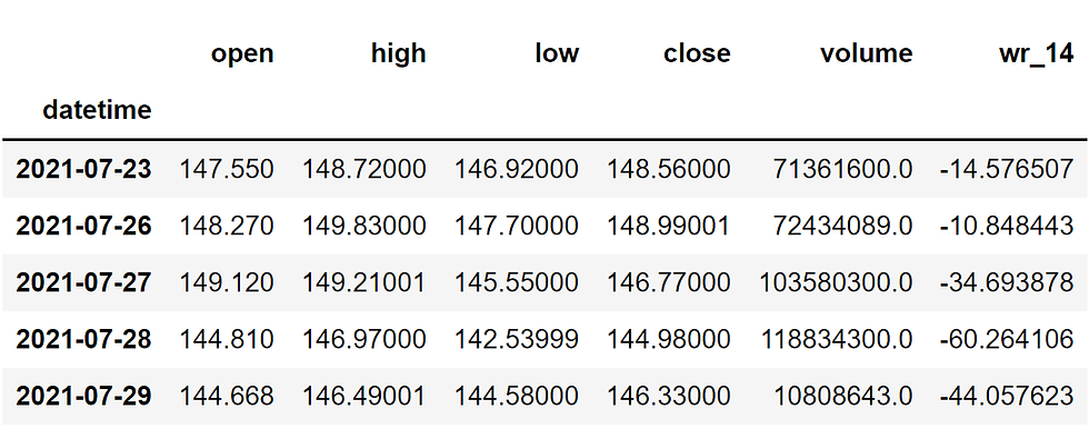
Code Explanation: We are first defining a function named ‘get_wr’ that takes a stock’s high price data (‘high’), low price data (‘low’), closing price data (‘close’), and the lookback period (‘period’) as parameters.
Inside the function, we are first determining the highest high over a specific lookback period timeframe with the help of the ‘rolling’ and ‘max’ functions provided by the Pandas package and stored it into the ‘highh’ variable. What the ‘rolling’ function performs is that it will take into account the n-period timeframe we specify and the ‘max’ function filters the maximum values present in the given dataframe.
Next, we are defining a variable named ‘lowl’ to store the lowest low over a specified lookback period timeframe which we determined using the ‘rolling’ and ‘min’ function (as the name suggests, filters the minimum values in the given dataframe) provided by the Pandas package.
Then, we are substituting the determined highest high and lowest low values into the formula we discussed before to calculate the values of Williams %R and stored it into the ‘wr’ variable. Finally, we are returning and calling the created function to store Apple’s Williams %R readings with 14 as the lookback period.
Step-4: MACD Calculation
In this step, we are going to calculate all the components of the MACD indicator from the extracted historical data of Apple.
# MACD CALCULATION

def get_macd(price, slow, fast, smooth):
    exp1 = price.ewm(span = fast, adjust = False).mean()
    exp2 = price.ewm(span = slow, adjust = False).mean()
    macd = pd.DataFrame(exp1 - exp2).rename(columns = {'close':'macd'})
    signal = pd.DataFrame(macd.ewm(span = smooth, adjust = False).mean()).rename(columns = {'macd':'signal'})
    hist = pd.DataFrame(macd['macd'] - signal['signal']).rename(columns = {0:'hist'})
    return macd, signal, hist

aapl['macd'] = get_macd(aapl['close'], 26, 12, 9)[0]
aapl['macd_signal'] = get_macd(aapl['close'], 26, 12, 9)[1]
aapl['macd_hist'] = get_macd(aapl['close'], 26, 12, 9)[2]
aapl = aapl.dropna()
aapl.tail()
Output:

Code Explanation: Firstly, we are defining a function named ‘get_macd’ that takes the stock’s price (‘prices’), length of the slow EMA (‘slow’), length of the fast EMA (‘fast’), and the period of the Signal line (‘smooth’).
Inside the function, we are first calculating the fast and slow length EMAs using the ‘ewm’ function provided by Pandas and stored them into the ‘ema1’ and ‘ema2’ variables respectively.
Next, we calculated the values of the MACD line by subtracting the slow length EMA from the fast length EMA and stored it into the ‘macd’ variable in the form of a Pandas dataframe. Followed by that, we defined a variable named ‘signal’ to store the values of the Signal line calculated by taking the EMA of the MACD line’s values (‘macd’) for a specified number of periods.
Then, we calculated the Histogram values by subtracting the MACD line’s values (‘macd’) from the Signal line’s values (‘signal’) and stored them into the ‘hist’ variable. Finally, we returning all the calculated values and called the created function to store Apple’s MACD components.
Step-5: Creating the Trading Strategy:
In this step, we are going to implement the discussed Williams %R and Moving Average Convergence/Divergence (MACD) combined trading strategy in python.
Python Implementation:
# TRADING STRATEGY

def implement_wr_macd_strategy(prices, wr, macd, macd_signal):
    buy_price = []
    sell_price = []
    wr_macd_signal = []
    signal = 0

    for i in range(len(wr)):
        if wr[i-1] > -50 and wr[i] < -50 and macd[i] > macd_signal[i]:
            if signal != 1:
                buy_price.append(prices[i])
                sell_price.append(np.nan)
                signal = 1
                wr_macd_signal.append(signal)
            else:
                buy_price.append(np.nan)
                sell_price.append(np.nan)
                wr_macd_signal.append(0)

        elif wr[i-1] < -50 and wr[i] > -50 and macd[i] < macd_signal[i]:
            if signal != -1:
                buy_price.append(np.nan)
                sell_price.append(prices[i])
                signal = -1
                wr_macd_signal.append(signal)
            else:
                buy_price.append(np.nan)
                sell_price.append(np.nan)
                wr_macd_signal.append(0)

        else:
            buy_price.append(np.nan)
            sell_price.append(np.nan)
            wr_macd_signal.append(0)

    return buy_price, sell_price, wr_macd_signal

buy_price, sell_price, wr_macd_signal = implement_wr_macd_strategy(aapl['close'], aapl['wr_14'], aapl['macd'], aapl['macd_signal'])
Code Explanation: First, we are defining a function named ‘wr_macd_strategy’ which takes the stock prices (‘prices’), Williams %R readings (‘wr’), MACD line readings (‘macd’), and the Signal line readings (‘macd_signal’) as parameters.
Inside the function, we are creating three empty lists (buy_price, sell_price, and wr_macd_signal) in which the values will be appended while creating the trading strategy.
After that, we are implementing the trading strategy through a for-loop. Inside the for-loop, we are passing certain conditions, and if the conditions are satisfied, the respective values will be appended to the empty lists. If the condition to buy the stock gets satisfied, the buying price will be appended to the ‘buy_price’ list, and the signal value will be appended as 1 representing to buy the stock. Similarly, if the condition to sell the stock gets satisfied, the selling price will be appended to the ‘sell_price’ list, and the signal value will be appended as -1 representing to sell the stock. Finally, we are returning the lists appended with values.
Then, we are calling the created function and stored the values into their respective variables.
Step-6: Creating our Position
In this step, we are going to create a list that indicates 1 if we hold the stock or 0 if we don’t own or hold the stock.
Python Implementation:
# POSITION

position = []
for i in range(len(wr_macd_signal)):
    if wr_macd_signal[i] > 1:
        position.append(0)
    else:
        position.append(1)

for i in range(len(aapl['close'])):
    if wr_macd_signal[i] == 1:
        position[i] = 1
    elif wr_macd_signal[i] == -1:
        position[i] = 0
    else:
        position[i] = position[i-1]

close_price = aapl['close']
wr = aapl['wr_14']
macd_line = aapl['macd']
signal_line = aapl['macd_signal']
wr_macd_signal = pd.DataFrame(wr_macd_signal).rename(columns = {0:'wr_macd_signal'}).set_index(aapl.index)
position = pd.DataFrame(position).rename(columns = {0:'wr_macd_position'}).set_index(aapl.index)

frames = [close_price, wr, macd_line, signal_line, wr_macd_signal, position]
strategy = pd.concat(frames, join = 'inner', axis = 1)

strategy.head()
Output:

Code Explanation: First, we are creating an empty list named ‘position’. We are passing two for-loops, one is to generate values for the ‘position’ list to just match the length of the ‘signal’ list. The other for-loop is the one we are using to generate actual position values.
Inside the second for-loop, we are iterating over the values of the ‘signal’ list, and the values of the ‘position’ list get appended concerning which condition gets satisfied. The value of the position remains 1 if we hold the stock or remains 0 if we sold or don’t own the stock. Finally, we are doing some data manipulations to combine all the created lists into one dataframe.
From the output being shown, we can see that in the first three rows our position in the stock has remained 1 (since there isn’t any change in the trading signal) but our position suddenly turned to 0 as we sold the stock when the trading signal represents a buy signal (-1). Our position will remain -1 until some changes in the trading signal occur. Now it’s time to do implement some backtesting processes!
Step-7: Backtesting
Before moving on, it is essential to know what backtesting is. Backtesting is the process of seeing how well our trading strategy has performed on the given stock data. In our case, we are going to implement a backtesting process for our Williams %R and MACD combined trading strategy over the Apple stock data.
Python Implementation:
# BACKTESTING

aapl_ret = pd.DataFrame(np.diff(aapl['close'])).rename(columns = {0:'returns'})
wr_macd_strategy_ret = []

for i in range(len(aapl_ret)):
    try:
        returns = aapl_ret['returns'][i] * strategy['wr_macd_position'][i]
        wr_macd_strategy_ret.append(returns)
    except:
        pass

wr_macd_strategy_ret_df = pd.DataFrame(wr_macd_strategy_ret).rename(columns = {0:'wr_macd_returns'})

investment_value = 100000
number_of_stocks = floor(investment_value / aapl['close'][0])
wr_macd_investment_ret = []

for i in range(len(wr_macd_strategy_ret_df['wr_macd_returns'])):
    returns = number_of_stocks * wr_macd_strategy_ret_df['wr_macd_returns'][i]
    wr_macd_investment_ret.append(returns)

wr_macd_investment_ret_df = pd.DataFrame(wr_macd_investment_ret).rename(columns = {0:'investment_returns'})
total_investment_ret = round(sum(wr_macd_investment_ret_df['investment_returns']), 2)
profit_percentage = floor((total_investment_ret / investment_value) * 100)
print(cl('Profit gained from the W%R MACD strategy by investing $100k in AAPL : {}'.format(total_investment_ret), attrs = ['bold']))
print(cl('Profit percentage of the W%R MACD strategy : {}%'.format(profit_percentage), attrs = ['bold']))
Output:
Profit gained from the W%R MACD strategy by investing $100k in AAPL : 1207459.27
Profit percentage of the W%R MACD strategy : 1207%
Code Explanation: First, we are calculating the returns of the Apple stock using the ‘diff’ function provided by the NumPy package and we have stored it as a dataframe into the ‘aapl_ret’ variable. Next, we are passing a for-loop to iterate over the values of the ‘aapl_ret’ variable to calculate the returns we gained from our RVI trading strategy, and these returns values are appended to the ‘wr_macd_strategy_ret’ list. Next, we are converting the ‘wr_macd_strategy_ret’ list into a dataframe and stored it into the ‘wr_macd_strategy_ret_df’ variable.
Next comes the backtesting process. We are going to backtest our strategy by investing a hundred thousand USD into our trading strategy. So first, we are storing the amount of investment into the ‘investment_value’ variable. After that, we are calculating the number of Apple stocks we can buy using the investment amount. You can notice that I’ve used the ‘floor’ function provided by the Math package because, while dividing the investment amount by the closing price of Apple stock, it spits out an output with decimal numbers. The number of stocks should be an integer but not a decimal number. Using the ‘floor’ function, we can cut out the decimals. Remember that the ‘floor’ function is way more complex than the ‘round’ function. Then, we are passing a for-loop to find the investment returns followed by some data manipulation tasks.
Finally, we are printing the total return we got by investing a hundred thousand into our trading strategy and it is revealed that we have made an approximate profit of one million and two hundred thousand USD in around ten-and-a-half years with a profit percentage of 1207%. That’s great! Now, let’s compare our returns with SPY ETF (an ETF designed to track the S&P 500 stock market index) returns.
Step-8: SPY ETF Comparison
This step is optional but it is highly recommended as we can get an idea of how well our trading strategy performs against a benchmark (SPY ETF). In this step, we will extract the SPY ETF data using the ‘get_historical_data’ function we created and compare the returns we get from the SPY ETF with our trading strategy returns on Apple.
You might have observed that in all of my algorithmic trading articles, I’ve compared the strategy results not with the S&P 500 market index itself but with the SPY ETF and this is because most of the stock data providers (like Twelve Data) don’t provide the S&P 500 index data. So, I have no other choice than to go with the SPY ETF. If you’re fortunate to get the S&P 500 market index data, it is recommended to use it for comparison rather than any ETF.
Python Implementation:
# SPY ETF COMPARISON

def get_benchmark(start_date, investment_value):
    spy = get_historical_data('SPY', start_date)['close']
    benchmark = pd.DataFrame(np.diff(spy)).rename(columns = {0:'benchmark_returns'})

    investment_value = investment_value
    number_of_stocks = floor(investment_value/spy[0])
    benchmark_investment_ret = []

    for i in range(len(benchmark['benchmark_returns'])):
        returns = number_of_stocks*benchmark['benchmark_returns'][i]
        benchmark_investment_ret.append(returns)

    benchmark_investment_ret_df = pd.DataFrame(benchmark_investment_ret).rename(columns = {0:'investment_returns'})
    return benchmark_investment_ret_df

benchmark = get_benchmark('2010-01-01', 100000)
investment_value = 100000
total_benchmark_investment_ret = round(sum(benchmark['investment_returns']), 2)
benchmark_profit_percentage = floor((total_benchmark_investment_ret/investment_value)*100)
print(cl('Benchmark profit by investing $100k : {}'.format(total_benchmark_investment_ret), attrs = ['bold']))
print(cl('Benchmark Profit percentage : {}%'.format(benchmark_profit_percentage), attrs = ['bold']))
print(cl('W%R MACD Strategy profit is {}% higher than the Benchmark Profit'.format(profit_percentage - benchmark_profit_percentage), attrs = ['bold']))
Output:
Benchmark profit by investing $100k : 288493.39
Benchmark Profit percentage : 288%
W%R MACD Strategy profit is 919% higher than the Benchmark Profit
Code Explanation: The code used in this step is almost similar to the one used in the previous backtesting step but, instead of investing in Apple, we are investing in SPY ETF by not implementing any trading strategies. From the output, we can see that our trading strategy has outperformed the SPY ETF by 919%. That’s awesome!
Final Thoughts!
After an immense process of crushing both theory and programming parts, we have successfully learned what the Williams %R and the Moving Average Convergence/Divergence is all about and built a trading strategy by combining both of these indicators using python that actually makes a profit.
Now it’s time to talk about areas of improvement. The first aspect is going to be building an even more complex trading strategy. Using two technical indicators doesn’t entail that our strategy is complex enough to beat the crazy market. So it is highly recommended to come up with new, innovative, and unconventional strategies and backtest them on various stocks with different timeframes and scenarios.
The next aspect is strategy evaluation. For those who don’t know what evaluation means in the realm of trading, it is the process of drawing practical insights from the trading strategy. In this article, we directly jumped to a conclusion that our strategy is profitable by just scrutinizing the returns or profits that have been made but there are numerous factors to be considered of. So, evaluating our trading strategy helps us in understanding it even better with more practical and realistic facts.
The final aspect is obviously risk management. It is the most common and sensitive term in the stock market and a must-implemented concept in a trading system. Just because we have not implemented it in this article, it doesn’t mean it is not that important and must be ensured that it has been deployed properly before taking the strategy into the real-world market.
The reason for not discussing these aspects in this article is because each concept is a whole new chapter in the trading space and cannot be fitted in just a small section of an article. With that being said, you’ve reached the end of the article. If you forgot to follow any of the coding parts, don’t worry. I’ve provided the full source code at the end of the article. Hope you learned something new and useful from this article.
Hang on! If you’re interested in algorithmic trading with Python, it is highly recommended to take the online program Algorithmic Trading for Everyone which is a specialization conducted by Quantra (a python platform for quantitative finance). This program is well-structured and designed in a fashion that makes both beginners and advanced users enjoy and follow along with the concepts more easily and efficiently.
Full code:
# IMPORTING PACKAGES

import numpy as np
import pandas as pd
import matplotlib.pyplot as plt
import requests
from math import floor
from termcolor import colored as cl

plt.style.use('fivethirtyeight')
plt.rcParams['figure.figsize'] = (20,10)

# EXTRACTING STOCK DATA

def get_historical_data(symbol, start_date):
    api_key = 'YOUR API KEY'
    api_url = f'https://api.twelvedata.com/time_series?symbol={symbol}&interval=1day&outputsize=5000&apikey={api_key}'
    raw_df = requests.get(api_url).json()
    df = pd.DataFrame(raw_df['values']).iloc[::-1].set_index('datetime').astype(float)
    df = df[df.index >= start_date]
    df.index = pd.to_datetime(df.index)
    return df

aapl = get_historical_data('AAPL', '2010-01-01')
aapl.tail()

# WILLIAMS %R CALCULATION

def get_wr(high, low, close, lookback):
    highh = high.rolling(lookback).max()
    lowl = low.rolling(lookback).min()
    wr = -100 * ((highh - close) / (highh - lowl))
    return wr

aapl['wr_14'] = get_wr(aapl['high'], aapl['low'], aapl['close'], 14)
aapl.tail()

# WILLIAMS %R PLOT

plot_data = aapl[aapl.index >= '2020-01-01']

ax1 = plt.subplot2grid((11,1), (0,0), rowspan = 5, colspan = 1)
ax2 = plt.subplot2grid((11,1), (6,0), rowspan = 5, colspan = 1)
ax1.plot(plot_data['close'], linewidth = 2)
ax1.set_title('AAPL CLOSING PRICE')
ax2.plot(plot_data['wr_14'], color = 'orange', linewidth = 2)
ax2.axhline(-20, linewidth = 1.5, linestyle = '--', color = 'grey')
ax2.axhline(-80, linewidth = 1.5, linestyle = '--', color = 'grey')
ax2.set_title('AAPL WILLIAMS %R 14')
plt.show()

# MACD CALCULATION

def get_macd(price, slow, fast, smooth):
    exp1 = price.ewm(span = fast, adjust = False).mean()
    exp2 = price.ewm(span = slow, adjust = False).mean()
    macd = pd.DataFrame(exp1 - exp2).rename(columns = {'close':'macd'})
    signal = pd.DataFrame(macd.ewm(span = smooth, adjust = False).mean()).rename(columns = {'macd':'signal'})
    hist = pd.DataFrame(macd['macd'] - signal['signal']).rename(columns = {0:'hist'})
    return macd, signal, hist

aapl['macd'] = get_macd(aapl['close'], 26, 12, 9)[0]
aapl['macd_signal'] = get_macd(aapl['close'], 26, 12, 9)[1]
aapl['macd_hist'] = get_macd(aapl['close'], 26, 12, 9)[2]
aapl = aapl.dropna()
aapl.tail()

# MACD PLOT

plot_data = aapl[aapl.index >= '2020-01-01']

def plot_macd(prices, macd, signal, hist):
    ax1 = plt.subplot2grid((11,1), (0,0), rowspan = 5, colspan = 1)
    ax2 = plt.subplot2grid((11,1), (6,0), rowspan = 5, colspan = 1)

    ax1.plot(prices)
    ax1.set_title('AAPL STOCK PRICES')
    ax2.plot(macd, color = 'grey', linewidth = 1.5, label = 'MACD')
    ax2.plot(signal, color = 'skyblue', linewidth = 1.5, label = 'SIGNAL')
    ax2.set_title('AAPL MACD 26,12,9')

    for i in range(len(prices)):
        if str(hist[i])[0] == '-':
            ax2.bar(prices.index[i], hist[i], color = '#ef5350')
        else:
            ax2.bar(prices.index[i], hist[i], color = '#26a69a')

    plt.legend(loc = 'lower right')

plot_macd(plot_data['close'], plot_data['macd'], plot_data['macd_signal'], plot_data['macd_hist'])

# TRADING STRATEGY

def implement_wr_macd_strategy(prices, wr, macd, macd_signal):
    buy_price = []
    sell_price = []
    wr_macd_signal = []
    signal = 0

    for i in range(len(wr)):
        if wr[i-1] > -50 and wr[i] < -50 and macd[i] > macd_signal[i]:
            if signal != 1:
                buy_price.append(prices[i])
                sell_price.append(np.nan)
                signal = 1
                wr_macd_signal.append(signal)
            else:
                buy_price.append(np.nan)
                sell_price.append(np.nan)
                wr_macd_signal.append(0)

        elif wr[i-1] < -50 and wr[i] > -50 and macd[i] < macd_signal[i]:
            if signal != -1:
                buy_price.append(np.nan)
                sell_price.append(prices[i])
                signal = -1
                wr_macd_signal.append(signal)
            else:
                buy_price.append(np.nan)
                sell_price.append(np.nan)
                wr_macd_signal.append(0)

        else:
            buy_price.append(np.nan)
            sell_price.append(np.nan)
            wr_macd_signal.append(0)

    return buy_price, sell_price, wr_macd_signal

buy_price, sell_price, wr_macd_signal = implement_wr_macd_strategy(aapl['close'], aapl['wr_14'], aapl['macd'], aapl['macd_signal'])

# TRADING SIGNALS PLOT

plt.plot(aapl['close'])
plt.plot(aapl.index, buy_price, marker = '^', markersize = 10, color = 'green')
plt.plot(aapl.index, sell_price, marker = 'v', markersize = 10, color = 'r')

# POSITION

position = []
for i in range(len(wr_macd_signal)):
    if wr_macd_signal[i] > 1:
        position.append(0)
    else:
        position.append(1)

for i in range(len(aapl['close'])):
    if wr_macd_signal[i] == 1:
        position[i] = 1
    elif wr_macd_signal[i] == -1:
        position[i] = 0
    else:
        position[i] = position[i-1]

close_price = aapl['close']
wr = aapl['wr_14']
macd_line = aapl['macd']
signal_line = aapl['macd_signal']
wr_macd_signal = pd.DataFrame(wr_macd_signal).rename(columns = {0:'wr_macd_signal'}).set_index(aapl.index)
position = pd.DataFrame(position).rename(columns = {0:'wr_macd_position'}).set_index(aapl.index)

frames = [close_price, wr, macd_line, signal_line, wr_macd_signal, position]
strategy = pd.concat(frames, join = 'inner', axis = 1)

strategy.head()

# BACKTESTING

aapl_ret = pd.DataFrame(np.diff(aapl['close'])).rename(columns = {0:'returns'})
wr_macd_strategy_ret = []

for i in range(len(aapl_ret)):
    try:
        returns = aapl_ret['returns'][i] * strategy['wr_macd_position'][i]
        wr_macd_strategy_ret.append(returns)
    except:
        pass

wr_macd_strategy_ret_df = pd.DataFrame(wr_macd_strategy_ret).rename(columns = {0:'wr_macd_returns'})

investment_value = 100000
number_of_stocks = floor(investment_value / aapl['close'][0])
wr_macd_investment_ret = []

for i in range(len(wr_macd_strategy_ret_df['wr_macd_returns'])):
    returns = number_of_stocks * wr_macd_strategy_ret_df['wr_macd_returns'][i]
    wr_macd_investment_ret.append(returns)

wr_macd_investment_ret_df = pd.DataFrame(wr_macd_investment_ret).rename(columns = {0:'investment_returns'})
total_investment_ret = round(sum(wr_macd_investment_ret_df['investment_returns']), 2)
profit_percentage = floor((total_investment_ret / investment_value) * 100)
print(cl('Profit gained from the W%R MACD strategy by investing $100k in AAPL : {}'.format(total_investment_ret), attrs = ['bold']))
print(cl('Profit percentage of the W%R MACD strategy : {}%'.format(profit_percentage), attrs = ['bold']))

# SPY ETF COMPARISON

def get_benchmark(start_date, investment_value):
    spy = get_historical_data('SPY', start_date)['close']
    benchmark = pd.DataFrame(np.diff(spy)).rename(columns = {0:'benchmark_returns'})

    investment_value = investment_value
    number_of_stocks = floor(investment_value/spy[0])
    benchmark_investment_ret = []

    for i in range(len(benchmark['benchmark_returns'])):
        returns = number_of_stocks*benchmark['benchmark_returns'][i]
        benchmark_investment_ret.append(returns)

    benchmark_investment_ret_df = pd.DataFrame(benchmark_investment_ret).rename(columns = {0:'investment_returns'})
    return benchmark_investment_ret_df

benchmark = get_benchmark('2010-01-01', 100000)

investment_value = 100000
total_benchmark_investment_ret = round(sum(benchmark['investment_returns']), 2)
benchmark_profit_percentage = floor((total_benchmark_investment_ret/investment_value)*100)
print(cl('Benchmark profit by investing $100k : {}'.format(total_benchmark_investment_ret), attrs = ['bold']))
print(cl('Benchmark Profit percentage : {}%'.format(benchmark_profit_percentage), attrs = ['bold']))
print(cl('W%R MACD Strategy profit is {}% higher than the Benchmark Profit'.format(profit_percentage - benchmark_profit_percentage), attrs = ['bold']))


Doesn't PREV.WR > -50 and CUR.WR < -50 indicate a downtrend? Why would we perform a buy signal? (MACD.L > SIGNAL.L is a buy signal...so that's ok.)
Interesting Article Nikhil
Good work Nikil. The write up has come out well and will be useful to stock traders to get maximum return.
Paramasivan
Williams%R
MACD
Synergistic advantages
Python implementation
even, evaluation means in the realm of trading ......
Suggestion on a online course for beginners as well as the experts....
Well-structured and useful one.
Good Nikhil
Thanks